7.1. Matrix Statistics
The Matrix Statistics procedure provides information on matrix data under the same assumptions as the regression procedures. This means that all column lengths must be equal and any rows containing at least one missing value are omitted.
It is possible to create interaction terms, dummy and lag/lead variables just as in Linear Regression, Stepwise Regression, Logistic Regression, Multinomial Regression, Poisson Regression and Cox Regression procedures. This feature provides summary statistics on the terms of the regression models selected or created. It also enables you to send the entire final raw data (X) matrix to the Output Medium, so that you can see the actual values of all terms in the model. In Stand-Alone Mode, this output can then be sent to the Data Processor and used as input data in other procedures if necessary.
7.1.1. Matrix Statistics Variable Selection
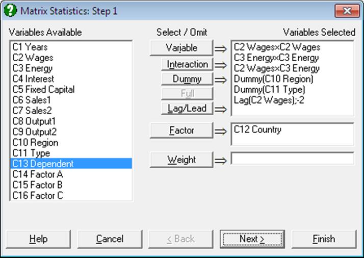
For further information on the tasks of the following buttons see 7.2.1.1. Linear Regression Variable Selection and 2.1.4. Creating Interaction, Dummy and Lag/Lead Variables.
Variable: Click on [Variable] to select a column containing continuous numeric data.
Interaction: Use this button to create variables, which are the products of existing numeric variables. If only one variable is highlighted, then the new variable will be the product of the selected variable by itself.
Dummy: This button is used to create n or n – 1 new dummy (or indicator) variables for a factor column containing n levels. It is possible to include all n levels in the analysis or to omit the first or the last level in order to remove the inherent over-parameterisation of the model.
Full: This button becomes activated when two or more categorical variables are highlighted. Like the [Dummy] button, it is also used to create dummy variables. The only difference is that this button will create all necessary dummy variables and their interactions to specify a complete model.
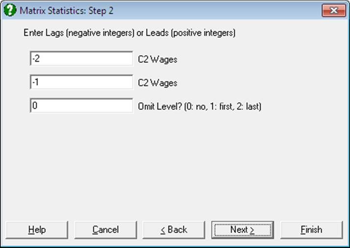
Lag/Lead: This button is used to create new variables by shifting the rows of an existing variable up or down. When a lag variable is specified then a further dialogue will ask for the number of lags (or leads) for each item selected. Negative integers represent the lags and positive integers the leads.
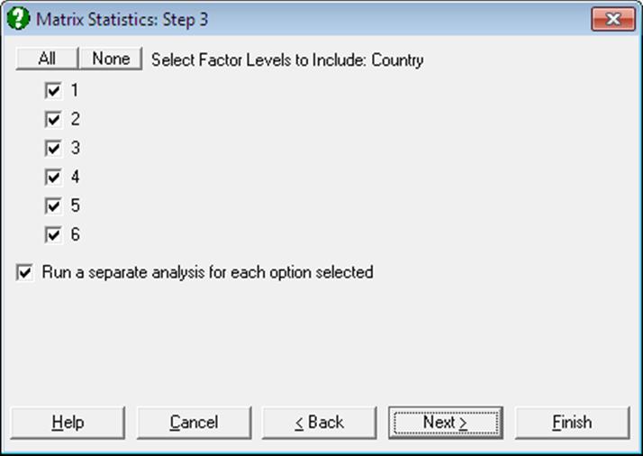
Factor: Selection of a factor variable is optional. It is possible to select an unlimited number of factor variables to define the rows to be included in the analysis. This allows you to analyse subsamples of rows (cases) without having to extract them by data manipulation first. When one or more factor columns are selected a further dialogue will ask you which factor levels to include. It is also possible to run a single analysis on all selected rows combined, or to run a separate analysis for each selection.
Weight: As in the Linear Regression procedure, a column may be selected as a weights variable. The program first normalises this column so that its sum is equal to the number of valid rows (after omitting missing rows), and then multiplies every row of the other selected columns by the square root of the corresponding row of the normalised weight column. The original data remains unchanged.
7.1.2. Matrix Statistics Output Options
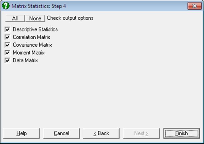
Descriptive Statistics: The following information on selected data columns is displayed in the form of a matrix: mean, standard deviation, standard error, variance, sum of squares, minimum and maximum.
This table is similar to the Data Processor’s Information output, except that the present output is produced under the assumptions outlined above. If the original data contains columns with equal lengths, it has no missing data, and a weight column is not selected, then the numbers in two outputs will be the same.
Correlation Matrix: Zero order (Pearson) Correlation Coefficients between all possible pairs of selected columns are computed. Among other uses, this option may be helpful in choosing variables for the Regression Analysis.
Covariance Matrix: Covariances between all possible pairs of selected columns are computed. Diagonal elements are variances and off-diagonal elements are covariances.
Moment Matrix: Second moments (sum of squared differences from the mean) between all possible pairs of selected columns are computed.
Data Matrix: Check this option to send the raw data matrix to Output Medium. This is most useful when interaction terms or dummy or lag/lead variables are included in the regression model and you wonder what the program does exactly. In Stand-Alone Mode, the matrix can then be sent to Data Processor and the generated variables used as input data in other procedures.
7.1.3. Matrix Statistics Examples
Example 1
Example 20.1b on p. 422 from Zar, J. H. (2010).
Open REGRESS, select Statistics 1 → Matrix Statistics and select temperature, cm, mm, min and ml (C1 to C5) as [Variable]s to obtain the following results:
Matrix Statistics
Valid Number of Cases: 33, 0 Omitted
Correlation Matrix
|
|
temperature |
cm |
mm |
min |
ml |
|
Temperature |
1.0000 |
0.3287 |
0.1677 |
0.0519 |
-0.7308 |
|
Cm |
0.3287 |
1.0000 |
-0.1455 |
0.1803 |
-0.2120 |
|
Mm |
0.1677 |
-0.1455 |
1.0000 |
0.2413 |
-0.0554 |
|
Min |
0.0519 |
0.1803 |
0.2413 |
1.0000 |
0.3127 |
|
Ml |
-0.7308 |
-0.2120 |
-0.0554 |
0.3127 |
1.0000 |
Example 2
Open DEMODATA, select Statistics 1 → Matrix Statistics and select the following terms in the model:
· Wages x Wages
· Energy x Energy
· Wages x Energy
· Dummy(Region)
· Dummy(Type)
· Lag(C2 Wages);0
· Lag(C2 Wages);0
On the next dialogue, enter -2 and 2 for the number of lags and 2 for the Omit Level? field. In the following results, the Data Matrix output is abbreviated for space considerations.
Matrix Statistics
Valid Number of Cases: 50, 8 Omitted
Descriptive Statistics
|
|
AVG |
STD |
SER |
VAR |
|
Wages x Wages |
10463.2380 |
2475.8040 |
350.1316 |
6129605.2550 |
|
Energy x Energy |
10263.4280 |
2774.2010 |
392.3313 |
7696191.0868 |
|
Wages x Energy |
10354.7937 |
2601.7470 |
367.9426 |
6769087.2265 |
|
Region = 1 |
0.2200 |
0.4185 |
0.0592 |
0.1751 |
|
2 |
0.5000 |
0.5051 |
0.0714 |
0.2551 |
|
Type = 1 |
0.3000 |
0.4629 |
0.0655 |
0.2143 |
|
Lag(C2 Wages);-2 |
100.1280 |
12.6974 |
1.7957 |
161.2237 |
|
Lag(C2 Wages);2 |
103.0340 |
12.3198 |
1.7423 |
151.7778 |
|
|
SUM |
SSQ |
MIN |
MAX |
|
Wages x Wages |
523161.9000 |
5774318129.726 |
6593.4400 |
13924.0000 |
|
Energy x Energy |
513171.3997 |
5644011072.654 |
6480.2500 |
14935.2841 |
|
Wages x Energy |
517739.6860 |
5692772923.285 |
6536.6000 |
14176.3600 |
|
Region = 1 |
11.0000 |
11.0000 |
0.0000 |
1.0000 |
|
2 |
25.0000 |
25.0000 |
0.0000 |
1.0000 |
|
Type = 1 |
15.0000 |
15.0000 |
0.0000 |
1.0000 |
|
Lag(C2 Wages);-2 |
5006.4000 |
509180.7800 |
81.2000 |
116.1000 |
|
Lag(C2 Wages);2 |
5151.7000 |
538237.3700 |
81.3000 |
121.2000 |
Correlation Matrix
|
|
Wages x Wages |
Energy x Energy |
Wages x Energy |
Region = 1 |
|
Wages x Wages |
1.0000 |
0.9607 |
0.9885 |
-0.1581 |
|
Energy x Energy |
0.9607 |
1.0000 |
0.9917 |
-0.1349 |
|
Wages x Energy |
0.9885 |
0.9917 |
1.0000 |
-0.1461 |
|
Region = 1 |
-0.1581 |
-0.1349 |
-0.1461 |
1.0000 |
|
2 |
0.0955 |
0.1285 |
0.1149 |
-0.5311 |
|
Type = 1 |
-0.0870 |
-0.0480 |
-0.0666 |
0.2845 |
|
Lag(C2 Wages);-2 |
0.9919 |
0.9694 |
0.9896 |
-0.1433 |
|
Lag(C2 Wages);2 |
0.9884 |
0.9140 |
0.9574 |
-0.1800 |
|
|
2 |
Type = 1 |
Lag(C2 Wages);-2 |
Lag(C2 Wages);2 |
|
Wages x Wages |
0.0955 |
-0.0870 |
0.9919 |
0.9884 |
|
Energy x Energy |
0.1285 |
-0.0480 |
0.9694 |
0.9140 |
|
Wages x Energy |
0.1149 |
-0.0666 |
0.9896 |
0.9574 |
|
Region = 1 |
-0.5311 |
0.2845 |
-0.1433 |
-0.1800 |
|
2 |
1.0000 |
-0.2182 |
0.1139 |
0.0769 |
|
Type = 1 |
-0.2182 |
1.0000 |
-0.0841 |
-0.0952 |
|
Lag(C2 Wages);-2 |
0.1139 |
-0.0841 |
1.0000 |
0.9688 |
|
Lag(C2 Wages);2 |
0.0769 |
-0.0952 |
0.9688 |
1.0000 |
Covariance Matrix
|
|
Wages x Wages |
Energy x Energy |
Wages x Energy |
Region = 1 |
|
Wages x Wages |
6129605.2550 |
6598743.5394 |
6367140.5020 |
-163.7585 |
|
Energy x Energy |
6598743.5394 |
7696191.0868 |
7157544.0234 |
-156.6458 |
|
Wages x Energy |
6367140.5020 |
7157544.0234 |
6769087.2265 |
-159.0871 |
|
Region = 1 |
-163.7585 |
-156.6458 |
-159.0871 |
0.1751 |
|
2 |
119.4400 |
180.0707 |
151.0527 |
-0.1122 |
|
Type = 1 |
-99.6882 |
-61.6220 |
-80.1629 |
0.0551 |
|
Lag(C2 Wages);-2 |
31180.0560 |
34145.7844 |
32690.9879 |
-0.7614 |
|
Lag(C2 Wages);2 |
30147.2970 |
31238.5588 |
30688.3630 |
-0.9280 |
|
|
2 |
Type = 1 |
Lag(C2 Wages);-2 |
Lag(C2 Wages);2 |
|
Wages x Wages |
119.4400 |
-99.6882 |
31180.0560 |
30147.2970 |
|
Energy x Energy |
180.0707 |
-61.6220 |
34145.7844 |
31238.5588 |
|
Wages x Energy |
151.0527 |
-80.1629 |
32690.9879 |
30688.3630 |
|
Region = 1 |
-0.1122 |
0.0551 |
-0.7614 |
-0.9280 |
|
2 |
0.2551 |
-0.0510 |
0.7306 |
0.4786 |
|
Type = 1 |
-0.0510 |
0.2143 |
-0.4943 |
-0.5431 |
|
Lag(C2 Wages);-2 |
0.7306 |
-0.4943 |
161.2237 |
151.5460 |
|
Lag(C2 Wages);2 |
0.4786 |
-0.5431 |
151.5460 |
151.7778 |
Moment Matrix
|
|
Wages x Wages |
Energy x Energy |
Wages x Energy |
Region = 1 |
|
Wages x Wages |
115486362.5945 |
113855458.4657 |
114584468.8253 |
2141.4290 |
|
Energy x Energy |
113855458.4657 |
112880221.4531 |
113290072.8809 |
2104.4413 |
|
Wages x Energy |
114584468.8253 |
113290072.8809 |
113855458.4657 |
2122.1492 |
|
Region = 1 |
2141.4290 |
2104.4413 |
2122.1492 |
0.2200 |
|
2 |
5348.6702 |
5308.1833 |
5325.4285 |
0.0000 |
|
Type = 1 |
3041.2770 |
3018.6389 |
3027.8784 |
0.1200 |
|
Lag(C2 Wages);-2 |
1078219.5494 |
1061119.3869 |
1068841.9538 |
21.2820 |
|
Lag(C2 Wages);2 |
1107613.6152 |
1088095.8276 |
1096970.4119 |
21.7580 |
|
|
2 |
Type = 1 |
Lag(C2 Wages);-2 |
Lag(C2 Wages);2 |
|
Wages x Wages |
5348.6702 |
3041.2770 |
1078219.5494 |
1107613.6152 |
|
Energy x Energy |
5308.1833 |
3018.6389 |
1061119.3869 |
1088095.8276 |
|
Wages x Energy |
5325.4285 |
3027.8784 |
1068841.9538 |
1096970.4119 |
|
Region = 1 |
0.0000 |
0.1200 |
21.2820 |
21.7580 |
|
2 |
0.5000 |
0.1000 |
50.7800 |
51.9860 |
|
Type = 1 |
0.1000 |
0.3000 |
29.5540 |
30.3780 |
|
Lag(C2 Wages);-2 |
50.7800 |
29.5540 |
10183.6156 |
10465.1034 |
|
Lag(C2 Wages);2 |
51.9860 |
30.3780 |
10465.1034 |
10764.7474 |
Data Matrix
|
|
Wages x Wages |
Energy x Energy |
Wages x Energy |
Region = 1 |
|
1 |
14689.4400 |
14234.8761 |
14460.3720 |
0.0000 |
|
2 |
14256.3600 |
14089.6900 |
14172.7800 |
1.0000 |
|
3 |
13924.0000 |
13667.9481 |
13795.3800 |
0.0000 |
|
4 |
13572.2500 |
13218.1009 |
13394.0050 |
0.0000 |
|
5 |
13317.1600 |
12210.2500 |
12751.7000 |
1.0000 |
|
… |
… |
… |
… |
… |
|
|
2 |
Type = 1 |
Lag(C2 Wages);-2 |
Lag(C2 Wages);2 |
|
1 |
0.0000 |
0.0000 |
118.0000 |
* |
|
2 |
0.0000 |
0.0000 |
116.5000 |
* |
|
3 |
1.0000 |
0.0000 |
115.4000 |
121.2000 |
|
4 |
0.0000 |
1.0000 |
114.9000 |
119.4000 |
|
5 |
0.0000 |
0.0000 |
114.8000 |
118.0000 |
|
… |
… |
… |
… |
… |