7.2.7. Multinomial Regression

The Multinomial Regression procedure (which is also known as Multinomial Logistic or Polytomous regression) is suitable for estimating models where the dependent variable is a categorical variable. If the dependent variable contains only two categories, its results are identical to that of Logistic Regression. Therefore, Multinomial Regression can be considered as an extension of Logistic Regression.

In Multinomial Regression, a set of coefficients are estimated for each category of the dependent variable. This makes its output format fundamentally different from other types of regression (see 7.2.7.3. Multinomial Regression Output Options). Since the estimated model is over-determined, the coefficients are scaled according to one of the categories. By default, the most frequent category is selected as the base category, though this can be changed by the user. The estimated coefficients are displayed relative to the base category and their exponentials are called Relative Risk Ratios.

Multinomial Regression is also closely related to Discriminant Analysis in the sense that both procedures are used to estimate the membership of cases to the groups defined by a categorical variable (see 8.2. Discriminant Analysis). Multinomial Regression should be preferred when the list of independent variables contains dummy variables. Discriminant Analysis is more powerful than Multinomial Regression when all independent variables are continuous and meet the assumptions of multivariate normality.

Predictions (interpolations) and multicollinearity are handled as in other regression options (see, for instance, 7.2.6. Logistic Regression). Predicted cases are identified by an asterisk in Classification by Case, Probabilities and Index Values output options (see 7.2.7.3. Multinomial Regression Output Options).

7.2.7.1. Multinomial Regression Model Description

The multinomial logistic function is an extension of the logit function discussed in Logit / Probit / Gompit (see 7.2.5.1. Logit / Probit / Gompit Model Description).

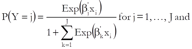
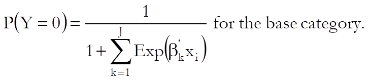
Let J + 1 be the number of distinct categories in the dependent variable and assume that the category 0 is selected as the base category. Then the probabilities given by the multinomial logistic function are:

where  is the vector of estimated coefficients for the j^th category and  is the i^th case (row) of the data matrix.

The relative risk ratio for case i relative to the base category is:

The logarithm of the likelihood function is given as:

and the first derivatives as:

where:

d_ij = 1 if Y_i = j and

d_ij = 0 otherwise.

A Newton-Raphson type maximum likelihood algorithm is employed to minimise the negative of the log likelihood function. The nature of this method implies that a solution (convergence) cannot always be achieved. In such cases, you are advised to edit the convergence parameters provided, in order to find the right levels for the particular problem at hand.

7.2.7.2. Multinomial Regression Variable Selection

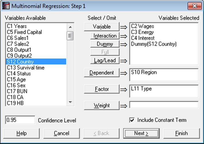
Like Logistic Regression, Multinomial Regression can be used to estimate models with or without a constant term, with or without weights and regressions can be run on a subset of cases as determined by the levels of an unlimited number of factor columns. An unlimited number of dependent variables (numeric or string) can be selected in order to run the same model on different dependent variables. It is also class="UniLink">2.1.4. Creating Interaction, Dummy and Lag/Lead Variables).

It is compulsory to select at least one categorical data column containing numeric or String Data as a dependent variable. When more than one dependent variable is selected, the analysis will be repeated as many times as the number of dependent variables, each time only changing the dependent variable and keeping the rest of selections unchanged.

A column containing numeric data can be selected as a weights column. Weights are frequency weights and all independent variables are multiplied by this column internally by the program.

An intermediate inputs dialogue is displayed next.

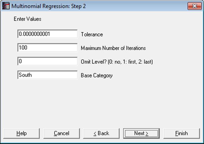
Tolerance: This value is used to control the sensitivity of nonlinear minimisation procedure employed. Under normal circumstances, you do not need to edit this value. If a convergence cannot be achieved, then larger values of this parameter can be tried by removing one or more zeros.

Maximum Number of Iterations: When convergence cannot be achieved with the default value of 100 function evaluations, a higher value can be tried.

Omit Level: This field will appear only when one or Dialogue. Three options are available; (0) do not omit any levels, (1) omit the first level and (2) omit the last level. When no levels are omitted, the model will usually be over-parameterised (see 2.1.4. Creating Interaction, Dummy and Lag/Lead Variables).

Base Category: By default, the most frequent category of the dependent variable is suggested as the base category. To scale the estimated coefficients according to a particular category, enter this category here. The Relative Risk Ratios will be relative to this category.

7.2.7.3. Multinomial Regression Output Options

When the calculations are finished an Output Options Dialogue will provide access to the following options.

Regression Results: The main regression output displays a table of estimated coefficients for each category of the dependent variable, except for the base category. Standard errors, Wald statistics, probability values and confidence intervals are also displayed for the estimated regression coefficients.

      Wald Statistic: This is defined as:

          

      and has a chi-square distribution with one degree of freedom.

      Confidence Intervals: The confidence intervals for regression coefficients are computed from:

           , i = 1, …, k, j = 1, …, J,

      where k is the number of independent variables in the model and each coefficient’s standard error, σ_ij, is the square root of the diagonal element of covariance matrix.

      -2 Log-Likelihood Initial Model: This is the value when all independent variables are excluded from the model:

           , i = 1, …, k, j = 1, …, J.

      -2 Log-Likelihood Final Model: This is ‑2 times the value of the log likelihood function when convergence is achieved.

      Pseudo R-squared: In Multinomial Regression, an r-squared statistic as in the OLS regression is not available. This is because Multinomial Regression employs an iterative maximum likelihood estimation method. Equivalent statistics to test the goodness of fit have been proposed using the initial (L₀) and maximum (L₁) likelihood values.

            McFadden:

                

           Adjusted McFadden:

                

           Cox & Snell:

                

           Nagelkerke:

                

      Likelihood Ratio: This is a test statistic for the null hypothesis that “all regression coefficients for independent variables are zero”. It is equal to ‑2 times the difference between the initial and final model likelihood values and has a chi-square distribution with kJ degrees of freedom (the number of independent variables in the model times the number of distinct categories in the independent variable excluding the base category).

Relative Risk Ratio:

      Values of the relative risk ratio indicate the influence of one unit change in a covariate on the regression.

           , i = 1, …, k, j = 1, …, J.

      The standard error of the relative risk ratio is:

          

      where σ_ij is the standard error of the i^th independent variable for the j^th category of the dependent variable. Coefficient confidence intervals are:

          

      which are simply the exponential of the coefficient confidence intervals.

Correlation Matrix of Regression Coefficients: This is a symmetric matrix with unity diagonal elements. The off-diagonal elements give correlations between the regression coefficients.

Covariance Matrix of Regression Coefficients: This is a symmetric matrix where diagonal elements are the square of parameter standard errors. The off-diagonal elements are covariances between the regression coefficients.

Classification by Group: A table is formed with rows and columns corresponding to observed and estimated group memberships respectively. Each cell displays the number of elements and its percentage with respect to the row total. The diagonal elements are the cases classified correctly and the off-diagonal elements are the misclassified cases.

Classification by Case: The observed and estimated group memberships are listed and pairs with disagreement are marked. The estimated group is the one with the highest probability level.

Probabilities: These are calculated as in the first two equations of Multinomial Regression Model Description. The predicted values are marked with two asterisks.

Index Values: These are the fitted values given as:

 for j = 0, …, J and i = 1, …, n.

The predicted values are marked with two asterisks.

7.2.7.4. Multinomial Regression Examples

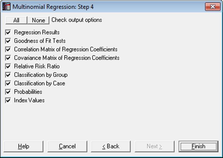
Open ANOVA and select Statistics 1 → Regression Analysis → Multinomial Regression. From the Variable Selection Dialogue select Period (C29) as [Dependent], Score (C26) as [Variable] and Noise (S30) as [Dummy]. On Step 2 dialogue enter 1 for Omit Level and leave other entries unchanged. Check all output options to obtain the following output. Some tables have been shortened.

Multinomial Regression

Regression Results

Valid Number of Cases: 54, 0 Omitted

Dependent Variable: Period

Base Category: 1

 

	Coefficient	Standard Error	Wald Statistic	Probability	Lower 95%	Upper 95%
Period = 2 Constant	4.2452	1.9258	4.8596	0.0275	0.4708	8.0196
Score	-0.0818	0.0358	5.2104	0.0225	-0.1519	-0.0116
Noise = Low	-0.4319	0.7490	0.3325	0.5642	-1.8999	1.0362
Period = 3 Constant	8.9299	2.3890	13.9723	0.0002	4.2476	13.6122
Score	-0.1924	0.0503	14.6346	0.0001	-0.2910	-0.0938
Noise = Low	-1.1811	0.9236	1.6352	0.2010	-2.9914	0.6292

 

-2 Log likelihood:
Initial Model =	118.6501
Final Model =	91.6682
Pseudo R-squared:
McFadden =	0.2274
Adjusted McFadden =	0.1768
Cox & Snell =	0.3933
Nagelkerke =	0.4424
Likelihood Ratio Statistic:
Chi-Square Statistic =	26.9820
Degrees of Freedom =	4
Right-Tail Probability =	0.0000

 

Relative Risk Ratio

	Relative Risk Ratio	Standard Error	Lower 95%	Upper 95%
Period = 2 Score	0.9215	0.0330	0.8590	0.9885
Noise = Low	0.6493	0.4863	0.1496	2.8184
Period = 3 Score	0.8249	0.0415	0.7475	0.9104
Noise = Low	0.3069	0.2835	0.0502	1.8761

 

Correlation Matrix of Regression Coefficients

	Period = 2 Constant	Score	Noise = Low	Period = 3 Constant	Score	Noise = Low
Period = 2 Constant	1.0000	-0.9642	-0.4271	0.6576	-0.5719	-0.2615
Score	-0.9642	1.0000	0.2573	-0.6220	0.5703	0.1609
Noise = Low	-0.4271	0.2573	1.0000	-0.2553	0.1441	0.5618
Period = 3 Constant	0.6576	-0.6220	-0.2553	1.0000	-0.9635	-0.4907
Score	-0.5719	0.5703	0.1441	-0.9635	1.0000	0.3417
Noise = Low	-0.2615	0.1609	0.5618	-0.4907	0.3417	1.0000

 

Covariance Matrix of Regression Coefficients

	Period = 2 Constant	Score	Noise = Low	Period = 3 Constant	Score	Noise = Low
Period = 2 Constant	3.7085	-0.0665	-0.6160	3.0251	-0.0554	-0.4651
Score	-0.0665	0.0013	0.0069	-0.0532	0.0010	0.0053
Noise = Low	-0.6160	0.0069	0.5610	-0.4568	0.0054	0.3886
Period = 3 Constant	3.0251	-0.0532	-0.4568	5.7072	-0.1158	-1.0828
Score	-0.0554	0.0010	0.0054	-0.1158	0.0025	0.0159
Noise = Low	-0.4651	0.0053	0.3886	-1.0828	0.0159	0.8531

 

Classification by Group

Observed\Predicted	1	2	3
1	12	4	2
	66.67%	22.22%	11.11%
2	7	5	6
	38.89%	27.78%	33.33%
3	0	5	13
	0.00%	27.78%	72.22%

 

Correctly Classified =

55.56%

 

Classification by Case

	Actual Group	Misclassified	Estimated Group	Probability
1	1	*	2	0.4327
2	1		1	0.4552
3	1		1	0.6290
4	2	*	3	0.4842
5	2	*	1	0.4283
6	2	*	1	0.5585
…	…	…	…	…

 

Probabilities

	1	2	3
1	0.2456	0.4327	0.3217
2	0.4552	0.4170	0.1279
3	0.6290	0.3251	0.0459
4	0.1413	0.3745	0.4842
5	0.4283	0.4258	0.1459
6	0.5585	0.3689	0.0726
7	0.0235	0.1661	0.8105
8	0.0953	0.3229	0.5819
9	0.2700	0.4383	0.2917
10	0.0716	0.2858	0.6426
11	0.1595	0.3896	0.4509
12	0.3744	0.4383	0.1873
13	0.0328	0.1969	0.7703
14	0.0953	0.3229	0.5819
15	0.2952	0.4417	0.2631
…	…	…	…

 

Index Values

	1	2	3
1	0.0000	0.5663	0.2698
2	0.0000	-0.0877	-1.2698
3	0.0000	-0.6600	-2.6169
4	0.0000	0.9751	1.2320
5	0.0000	-0.0059	-1.0773
6	0.0000	-0.4147	-2.0396
7	0.0000	1.9561	3.5414
8	0.0000	1.2204	1.8094
9	0.0000	0.4846	0.0774
10	0.0000	1.3839	2.1943
11	0.0000	0.8934	1.0396
12	0.0000	0.1576	-0.6924
13	0.0000	1.7926	3.1565
14	0.0000	1.2204	1.8094
15	0.0000	0.4028	-0.1151
…	…	…	…