7.2.8. Poisson Regression
The Poisson Regression procedure is suitable for models where the dependent variable is a frequency (count) variable consisting of nonnegative integers. The exponential of estimated regression coefficients are called Incidence Rate Ratios, which give the estimated rate at which events occur. This rate can be multiplied by an Exposure variable to obtain the expected frequencies, which enters the model with a coefficient constrained as 1.
Predictions (interpolations) and multicollinearity are handled as in other regression options (see, for instance, Logistic Regression). Predicted cases are identified by an asterisk in Case (Diagnostic) Statistics output options (see 7.2.8.3. Poisson Regression Output Options). The spreadsheet Reg function (see 3.4.2.6.3. UNISTAT Functions) will give the natural log of predicted values, which should be exponentiated to obtain the expected frequencies.
7.2.8.1. Poisson Regression Model Description
Poisson Regression assumes that actual frequencies yi are drawn from a Poisson distribution with parameters λi, i = 1, …, n. The associated probabilities are given as:
![]()
where:
![]()
is known as the loglinear model.
The logarithm of the likelihood function is given as:
![]()
and the first derivatives are:
![]()
A Newton-Raphson type maximum likelihood algorithm is employed to minimise the negative of the log likelihood function. The nature of this method implies that a solution (convergence) cannot always be achieved. In such cases, you are advised to edit the convergence parameters provided and try again.
7.2.8.2. Poisson Regression Variable Selection
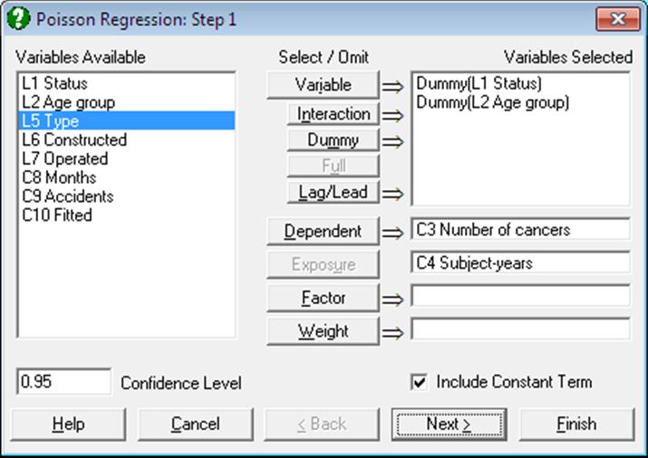
As in other regression procedures, Poisson Regression can be used to estimate models with or without a constant term, with or without weights and regressions can be run on a subset of cases as determined by the levels of an unlimited number of factor columns. An unlimited number of dependent variables can be selected in order to run the same model on different dependent variables. It is also possible to include interaction terms, dummy and lag/lead variables in the model, without having to create them as spreadsheet columns first (see 2.1.4. Creating Interaction, Dummy and Lag/Lead Variables).
It is compulsory to select at least one numeric data column containing frequency counts as a dependent variable. When more than one dependent variable is selected, the analysis will be repeated as many times as the number of dependent variables, each time only changing the dependent variable and keeping the rest of selections unchanged.
A column containing numeric data can be selected as a weights column. Weights are frequency weights and all independent variables are multiplied by this column internally by the program.
An intermediate inputs dialogue is displayed next.
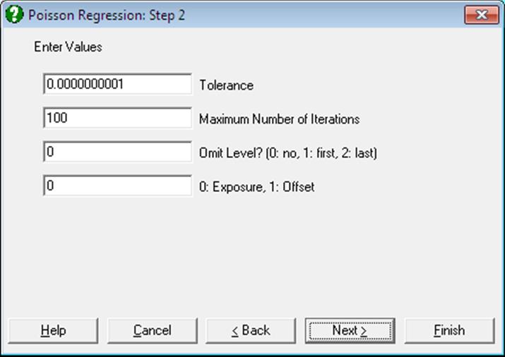
Tolerance: This value is used to control the sensitivity of nonlinear minimisation procedure employed. Under normal circumstances, you do not need to edit this value. If convergence cannot be achieved, then larger values of this parameter can be tried by removing one or more zeros.
Maximum Number of Iterations: When convergence cannot be achieved with the default value of 100 function evaluations, a higher value can be tried.
Omit Level: This field will appear only when one or more dummy variables have been included in the model from the Variable Selection Dialogue. Three options are available; (0) do not omit any levels, (1) omit the first level and (2) omit the last level. When no levels are omitted, the model will usually be over-parameterised (see 2.1.4. Creating Interaction, Dummy and Lag/Lead Variables).
Exposure / Offset: This field will appear only if a column has been assigned the task of [Exposure] in Variable Selection Dialogue. When the value of this field 0 the variable selected (E) will enter the model as Exposure:
![]()
and for any other value it will enter the model as Offset:
![]()
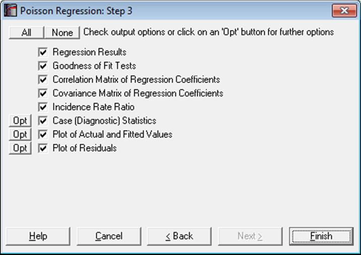
7.2.8.3. Poisson Regression Output Options
The Actual and Fitted Values, Residuals and Confidence Intervals for Mean and Actual Y Values options that existed in earlier versions of UNISTAT have now been merged with the Case (Diagnostic) Statistics option. See 7.2.1.2.2. Linear Regression Case Output.
Regression Results: The main regression output displays a table of estimated coefficients for each category of the dependent variable, except for the base category. Standard errors, Wald statistics, probability values and confidence intervals are also displayed for the estimated regression coefficients.
Wald Statistic: This is defined as:
![]()
and has a chi-square distribution with one degree of freedom.
Confidence Intervals: The confidence intervals for regression coefficients are computed from:
![]()
where k is the number of independent variables in the model and each coefficient’s standard error, σi, is the square root of the diagonal element of covariance matrix.
Goodness of Fit Tests: See 7.2.6.4.1. Logistic Regression Results for details.
Correlation Matrix of Regression Coefficients: This is a symmetric matrix with unity diagonal elements. The off-diagonal elements give correlations between the regression coefficients.
Covariance Matrix of Regression Coefficients: This is a symmetric matrix where diagonal elements are the square of parameter standard errors. The off-diagonal elements are covariances between the regression coefficients.
Incidence Rate Ratio: Values of the incidence rate ratio indicate the influence of one unit change in a covariate on the regression.
![]()
The standard error of the incidence rate ratio is:
![]()
where σi is the standard error of the ith independent variable for the jth category of the dependent variable. Coefficient confidence intervals are:
![]()
which are simply the exponential of the coefficient confidence intervals.
Case (Diagnostic) Statistics: Case statistics are useful to determine the influence of individual observations on the overall fit of the model. For further information see 7.2.1.2.2. Linear Regression Case Output.
Statistics available under this option are defined as follows.
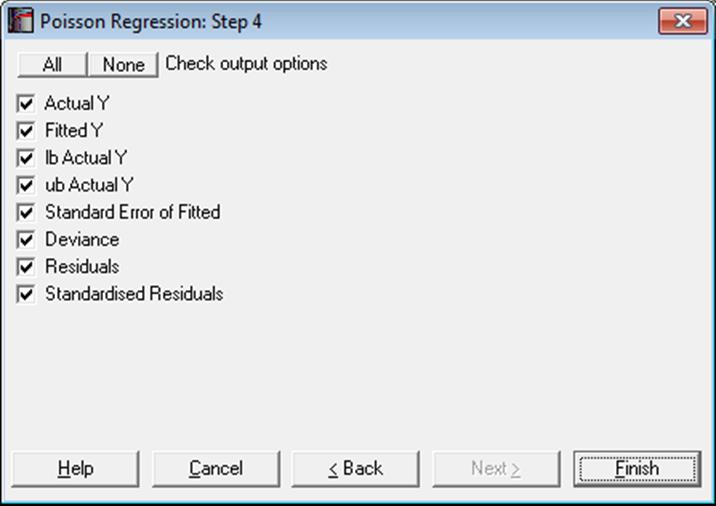
Actual Y: Observed values of the dependent variable.
Fitted Y: Also known as expected values:
![]()
Standard Error of Fitted:
![]()
Confidence Intervals of Fitted:
![]()
Deviance:
![]()
Residuals:
![]()
Standardised Residuals:
![]()
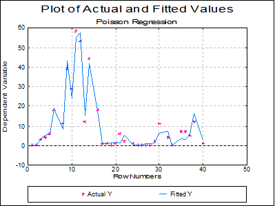
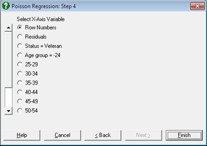
Plot of Actual and Fitted Values: Select this option to plot actual and fitted Y values against row numbers (index), residuals or against any independent variable. A further dialogue will enable you to choose the X-axis variable from a list.
By default, a line graph of the two series is plotted. However, since this procedure (like the plot of residuals) uses the X-Y Plots engine, it has almost all controls and options available for X-Y Plots, except for error bars and right Y-axes.
The data points on the graph will also respond to the right mouse button in the way X-Y Plots does; the point is highlighted, a panel displays information about the point and in Stand-Alone Mode, the row of the spreadsheet containing the data point is also highlighted (a procedure which is also known as Brushing or Point identification). While the point is highlighted you can press <Delete> to omit the particular row containing the point. The entire Regression Analysis will be run again without the deleted row. If you want to restore the original regression, you will need to take one of the following two actions depending on the way you run UNISTAT:
1. In Stand-Alone Mode, go back to the Data Processor and delete or deactivate the Select Row column created by the program.
2. In Excel Add-In Mode, highlight a different block of data to remove the effect of the internal Select Row column.
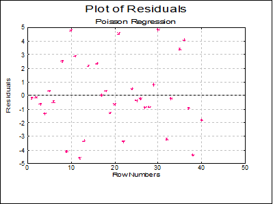
Plot of Residuals: Residuals can be plotted against row numbers (index), fitted values or against any independent variable. A further dialogue will enable you to choose the X-axis variable from a list containing Row Numbers, Fitted Values and all independent variables.
By default a scatter graph of residuals is plotted. For more information on available options see Plot of Actual and Fitted Values above.
7.2.8.4. Poisson Regression Examples
Example 1
Example 14.4 on p. 501 Armitage & Berry (2002). The aim is to assess whether there is a significant difference in cancer risk between veterans and non-veterans. The servicemen are divided into 11 age groups and their experience is given in terms of subject-years.
Open POISSON and select Statistics 1 → Regression Analysis → Poisson Regression. Select Status and Age group (L1 and L2) as [Dummy], Number of cancers (C3) as [Dependent] and Subject-years (C4) as [Exposure]. On Step 2 dialogue enter 1 for Omit Level and leave other entries unchanged. Uncheck all output options except for Regression Results and click [Finish].
Armitage and Berry include the logarithm of the Subject-years variable in the model as an Offset variable, which is equivalent to an Exposure variable.
Regression results show that the p-value of Status = Veteran variable is 0.9493. As this is much greater than 5%, we can conclude that there is no significant difference in cancer risk between veterans and non-veterans.
Poisson Regression
Dependent Variable: Number of cancers
Exposure: Subject-years
Valid Number of Cases: 22, 0 Omitted
Regression Results
|
|
Coeffi cient |
Standard Error |
Wald Statistic |
Signifi cance |
Lower 95% |
Upper 95% |
|
Constant |
-9.3248 |
0.2045 |
2079.0648 |
0.0000 |
-9.7257 |
-8.9240 |
|
Status = Veteran |
-0.0035 |
0.0555 |
0.0040 |
0.9493 |
-0.1123 |
0.1052 |
|
Age group = 25-29 |
0.6793 |
0.2325 |
8.5373 |
0.0035 |
0.2236 |
1.1350 |
|
30-34 |
1.3711 |
0.2177 |
39.6626 |
0.0000 |
0.9444 |
1.7978 |
|
35-39 |
1.9396 |
0.2121 |
83.6581 |
0.0000 |
1.5240 |
2.3553 |
|
40-44 |
2.0343 |
0.2161 |
88.6203 |
0.0000 |
1.6108 |
2.4579 |
|
45-49 |
2.7266 |
0.2222 |
150.5414 |
0.0000 |
2.2910 |
3.1621 |
|
50-54 |
3.2029 |
0.2206 |
210.7121 |
0.0000 |
2.7704 |
3.6353 |
|
55-59 |
3.7162 |
0.2178 |
291.1924 |
0.0000 |
3.2894 |
4.1430 |
|
60-64 |
4.0927 |
0.2177 |
353.4845 |
0.0000 |
3.6660 |
4.5193 |
|
65-69 |
4.2362 |
0.2242 |
356.9375 |
0.0000 |
3.7967 |
4.6757 |
|
70- |
4.3637 |
0.2274 |
368.3262 |
0.0000 |
3.9181 |
4.8094 |
Example 2
Example 19.21 on p. 932 Greene (1997). The number of accidents per service month is given for a sample of ship types. There are five types of ships constructed in four different time periods and observed in two time periods.
Open POISSON and select Statistics 1 → Regression Analysis → Poisson Regression. From the Variable Selection Dialogue select Type, Constructed and Operated (C5-C7) as [Dummy], Accidents (C9) as [Dependent] and Months (C8) as [Exposure]. On Step 2 dialogue enter 1 for Omit Level and leave other entries unchanged. Check all output options to obtain the following output. Some tables have been shortened to save space.
Poisson Regression
Dependent Variable: Accidents
Exposure: Months
Valid Number of Cases: 34, 6 Omitted
Regression Results
|
|
Coeffi cient |
Standard Error |
Wald Statistic |
Signi ficance |
Lower 95% |
Upper 95% |
|
Constant |
-6.4029 |
0.2175 |
866.444 |
0.0000 |
-6.8292 |
-5.9765 |
|
Type = Type B |
-0.5447 |
0.1776 |
9.4055 |
0.0022 |
-0.8928 |
-0.1966 |
|
Type C |
-0.6888 |
0.3290 |
4.3818 |
0.0363 |
-1.3337 |
-0.0439 |
|
Type D |
-0.0743 |
0.2906 |
0.0654 |
0.7981 |
-0.6438 |
0.4952 |
|
Type E |
0.3205 |
0.2358 |
1.8485 |
0.1740 |
-0.1415 |
0.7826 |
|
Constructed = C 65-69 |
0.6958 |
0.1497 |
21.6190 |
0.0000 |
0.4025 |
0.9892 |
|
C 70-74 |
0.8175 |
0.1698 |
23.1665 |
0.0000 |
0.4846 |
1.1503 |
|
C 75-79 |
0.4450 |
0.2332 |
3.6397 |
0.0564 |
-0.0122 |
0.9021 |
|
Operated = O 75-79 |
0.3839 |
0.1183 |
10.5357 |
0.0012 |
0.1521 |
0.6156 |
Goodness of Fit Tests
|
|
-2 Log likelihood |
|
Initial Model |
244.1948 |
|
Final Model |
136.8291 |
|
|
Chi-Square Statistic |
Degrees of Freedom |
Right-Tail Probability |
|
Pearson |
38.9626 |
24 |
0.0276 |
|
Likelihood Ratio |
107.3657 |
8 |
0.0000 |
|
|
Pseudo R-squared |
|
McFadden |
0.4397 |
|
Adjusted McFadden |
0.3660 |
|
Cox & Snell |
0.9575 |
|
Nagelkerke |
0.9582 |
Correlation Matrix of Regression Coefficients
|
|
Constant |
Type = Type B |
Type C |
Type D |
Type E |
|
Constant |
1.0000 |
-0.8115 |
-0.3783 |
-0.3706 |
-0.4680 |
|
Type = Type B |
-0.8115 |
1.0000 |
0.4331 |
0.4469 |
0.5698 |
|
Type C |
-0.3783 |
0.4331 |
1.0000 |
0.2377 |
0.3132 |
|
Type D |
-0.3706 |
0.4469 |
0.2377 |
1.0000 |
0.3349 |
|
Type E |
-0.4680 |
0.5698 |
0.3132 |
0.3349 |
1.0000 |
|
Constructed = C 65-69 |
-0.4847 |
0.0862 |
0.0360 |
0.0277 |
-0.0052 |
|
C 70-74 |
-0.5509 |
0.2722 |
0.0458 |
0.0284 |
-0.0377 |
|
C 75-79 |
-0.4015 |
0.2285 |
0.0968 |
-0.0962 |
0.0476 |
|
Operated = O 75-79 |
-0.2164 |
0.0256 |
-0.0030 |
-0.0047 |
0.0263 |
|
|
Constructed = C 65-69 |
C 70-74 |
C 75-79 |
Operated = O 75-79 |
|
Constant |
-0.4847 |
-0.5509 |
-0.4015 |
-0.2164 |
|
Type = Type B |
0.0862 |
0.2722 |
0.2285 |
0.0256 |
|
Type C |
0.0360 |
0.0458 |
0.0968 |
-0.0030 |
|
Type D |
0.0277 |
0.0284 |
-0.0962 |
-0.0047 |
|
Type E |
-0.0052 |
-0.0377 |
0.0476 |
0.0263 |
|
Constructed = C 65-69 |
1.0000 |
0.6337 |
0.4758 |
-0.1196 |
|
C 70-74 |
0.6337 |
1.0000 |
0.5494 |
-0.2629 |
|
C 75-79 |
0.4758 |
0.5494 |
1.0000 |
-0.3150 |
|
Operated = O 75-79 |
-0.1196 |
-0.2629 |
-0.3150 |
1.0000 |
Covariance Matrix of Regression Coefficients
|
|
Constant |
Type = Type B |
Type C |
Type D |
Type E |
|
Constant |
0.0473 |
-0.0314 |
-0.0271 |
-0.0234 |
-0.0240 |
|
Type = Type B |
-0.0314 |
0.0315 |
0.0253 |
0.0231 |
0.0239 |
|
Type C |
-0.0271 |
0.0253 |
0.1083 |
0.0227 |
0.0243 |
|
Type D |
-0.0234 |
0.0231 |
0.0227 |
0.0844 |
0.0229 |
|
Type E |
-0.0240 |
0.0239 |
0.0243 |
0.0229 |
0.0556 |
|
Constructed = C 65-69 |
-0.0158 |
0.0023 |
0.0018 |
0.0012 |
-0.0002 |
|
C 70-74 |
-0.0204 |
0.0082 |
0.0026 |
0.0014 |
-0.0015 |
|
C 75-79 |
-0.0204 |
0.0095 |
0.0074 |
-0.0065 |
0.0026 |
|
Operated = O 75-79 |
-0.0056 |
0.0005 |
-0.0001 |
-0.0002 |
0.0007 |
|
|
Constructed = C 65-69 |
C 70-74 |
C 75-79 |
Operated = O 75-79 |
|
Constant |
-0.0158 |
-0.0204 |
-0.0204 |
-0.0056 |
|
Type = Type B |
0.0023 |
0.0082 |
0.0095 |
0.0005 |
|
Type C |
0.0018 |
0.0026 |
0.0074 |
-0.0001 |
|
Type D |
0.0012 |
0.0014 |
-0.0065 |
-0.0002 |
|
Type E |
-0.0002 |
-0.0015 |
0.0026 |
0.0007 |
|
Constructed = C 65-69 |
0.0224 |
0.0161 |
0.0166 |
-0.0021 |
|
C 70-74 |
0.0161 |
0.0288 |
0.0218 |
-0.0053 |
|
C 75-79 |
0.0166 |
0.0218 |
0.0544 |
-0.0087 |
|
Operated = O 75-79 |
-0.0021 |
-0.0053 |
-0.0087 |
0.0140 |
Incidence Rate Ratio
|
|
Incidence Rate Ratio |
Standard Error |
Lower 95% |
Upper 95% |
|
Type = Type B |
0.5800 |
0.1030 |
0.4095 |
0.8215 |
|
Type C |
0.5022 |
0.1652 |
0.2635 |
0.9571 |
|
Type D |
0.9284 |
0.2697 |
0.5253 |
1.6408 |
|
Type E |
1.3779 |
0.3248 |
0.8680 |
2.1871 |
|
Constructed = C 65-69 |
2.0054 |
0.3001 |
1.4956 |
2.6890 |
|
C 70-74 |
2.2647 |
0.3846 |
1.6235 |
3.1592 |
|
C 75-79 |
1.5604 |
0.3640 |
0.9879 |
2.4648 |
|
Operated = O 75-79 |
1.4679 |
0.1736 |
1.1642 |
1.8509 |
Case (Diagnostic) Statistics
|
|
Actual Y |
Fitted Y |
95% lb Actual Y |
95% ub Actual Y |
Standard Error of Fitted |
|
1 |
0.0000 |
0.2104 |
-0.2159 |
0.6367 |
0.2175 |
|
2 |
0.0000 |
0.1532 |
-0.2858 |
0.5922 |
0.2240 |
|
3 |
3.0000 |
3.6382 |
3.2553 |
4.0210 |
0.1953 |
|
… |
… |
… |
… |
… |
… |
|
|
Deviance |
Residuals |
Standardised Residuals |
|
1 |
0.4208 |
-0.2104 |
-0.4587 |
|
2 |
0.3064 |
-0.1532 |
-0.3914 |
|
3 |
0.1191 |
-0.6382 |
-0.3346 |
|
… |
… |
… |
… |