7.2.6. Logistic Regression
The Logistic Regression procedure is suitable for estimating Linear Regression models when the dependent variable is a binary (or dichotomous) variable, that is, it consists of two values such as Yes or No, or in general 0 and 1. In such cases, where the dependent variable has an underlying binomial distribution (and thus the predicted Y values should lie between 0 and 1) the Linear Regression procedure cannot be employed.
Like Linear Regression, Logistic Regression can be used to estimate models with or without a constant term and regressions may be run on a subset of cases as determined by the levels of an unlimited number of factor columns. An unlimited number of dependent variables (numeric or string) can be selected in order to run the same model on different dependent variables. It is also possible to include interaction terms, dummy and lag/lead variables in the model, without having to create them as spreadsheet columns first.
Logistic Regression is closely related to Logit / Probit / Gompit. For a brief discussion of similarities and differences of these two procedures see 7.2.5. Logit / Probit / Gompit.
A comprehensive implementation of ROC (Receiver Operating Characteristic) analysis is included in the Logistic Regression procedure. The two output options Classification by Group and ROC Analysis, as well as the two graphics options, will provide a complete ROC analysis output. It is possible to compute AUC (area under the curve) and plot ROC curves with covariates and plot multiple ROC curves with multiple comparisons between AUCs.
7.2.6.1. Logistic Regression Model Description
Logistic Regression employs the logit model as explained in Logit / Probit / Gompit (see 7.2.5.1. Logit / Probit / Gompit Model Description). However, the log of likelihood function for the logistic model can be expressed more explicitly as:
![]()
with first derivatives:
![]()
where:
![]()
7.2.6.2. Logistic Regression Variable Selection
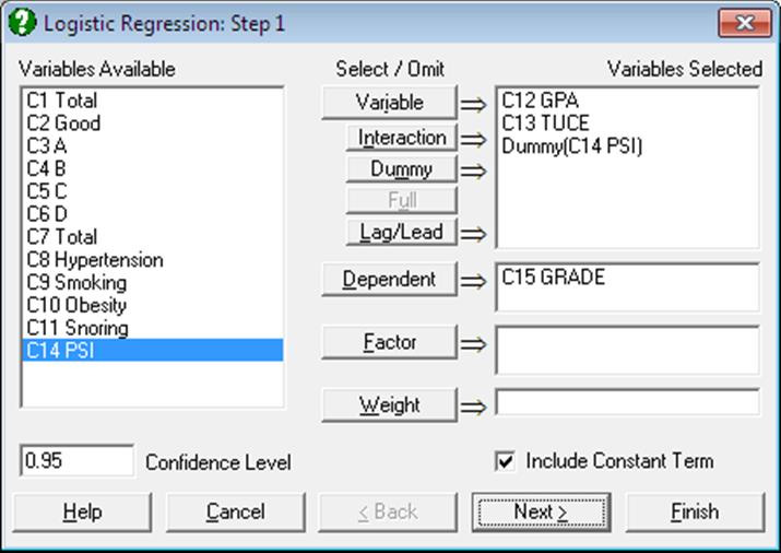
As in Linear Regression, it is possible to create interaction terms, dummy variables, lag/lead terms, select multiple dependent variables (see 2.1.4. Creating Interaction, Dummy and Lag/Lead Variables) and run regressions on subsamples defined by several factor columns with or without weights (see 7.2.1.1. Linear Regression Variable Selection).
It is compulsory to select at least one column containing numeric or String Data as a dependent variable. The program encodes the dependent variable internally such that, by default, the minimum value that occurs in the column is 0 and the rest are 1. It is possible to reverse this condition and encode the maximum of the dependent variable as 0 and the rest of the values as 1 using the Dependent Variable Encoding control in the Intermediate Inputs dialogue.
In case a categorical variable is not selected as the dependent variable, there may be too few 0s and too many 1s in the encoded dependent variable and convergence may not be achieved.
When more than one dependent variable is selected, the analysis will be repeated as many times as the number of dependent variables, each time only changing the dependent variable and keeping the rest of selections unchanged.
When more than one independent variable is selected, you will be presented with the option to run a single analysis (see 7.2.6.3. Logistic Regression Intermediate Inputs) including all independent variables or to run a separate regression for each independent variable, while holding the dependent variable unchanged. The primary use of this option is to compare the areas enclosed under the ROC curves for each independent variable.
A column containing numeric data can be selected as a weights column. Unlike the Linear Regression procedure, however, weights here are frequency weights. All independent variables are multiplied by this column internally by the program.
7.2.6.3. Logistic Regression Intermediate Inputs
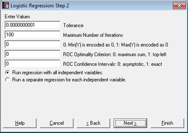
The number and kind of controls that appear on this dialogue depend on the selections made in the previous dialogue. For instance, if a dummy or lag variable was created, the dialogue will display one or more other boxes (see 2.1.4. Creating Interaction, Dummy and Lag/Lead Variables). The specific tasks of these controls are as follows:
Tolerance: This value is used to control the sensitivity of nonlinear minimisation procedure employed. Under normal circumstances, you do not need to edit this value. If convergence cannot be achieved, then larger values of this parameter can be tried by removing one or more zeros.
Maximum Number of Iterations: When convergence cannot be achieved with the default value of 100 function evaluations, a higher value can be tried.
Dependent Variable Encoding: By default, the program will internally encode the dependent variable values such that the minimum is 0 and the rest of the values are 1. If one is entered into this box, the program will encode the maximum value as 0 and the rest as 1.
Making a change in this control will normally reverse the signs of the estimated coefficients and will affect other output as well. If your aim in changing this control is to obtain the correct 2 x 2 table where the maximum value of the dependent variable corresponds to a positive state, e.g. the presence of a disease or vice versa, this can be done in the Output Options Dialogue more efficiently, without affecting the estimated coefficients and other output.
ROC Optimality Criterion: In Logistic Regression, the fitted Y is a continuous variable consisting of probability values. The estimated group membership (in terms of 0 and 1) is dependent on a critical cut-off probability which is also called the Classification threshold probability. The estimated group membership is 0 for any case with an estimated probability (fitted Y value) less than this critical probability and it is 1 otherwise.
The user is allowed to change this default value manually to play different what-if scenarios. The Classification threshold probability is estimated by the program using one of the following two methods:
Maximum sum of sensitivity and specificity: This is also known as the Youden’s index and represents the point on the curve furthest away from the 45º line. It is defined as:
Max(Sensitivity + Specificity)
Point nearest to the top-left corner of ROC plot: This is given as:
Min((1 – Sensitivity)^2 + (1- Specificity)^2)
The estimated Classification threshold probability can be edited to observe the effect of different cut-off values on the 2 x 2 Table and Statistics For Diagnostic Tests output..
ROC Confidence Intervals: The ROC Table output option (see 7.2.6.4.4. ROC Analysis) can display all cases for a large number of test statistics together with their confidence intervals. Here you can choose the type of confidence intervals as:
0: Asymptotic normal (Wald), or
1: Exact binomial (Clopper-Pearson).
Run regression with all independent variables: This is the default option and produces one set of output with all independent variables included.
Run a separate regression for each independent variable: It is possible to run a separate regression for each independent variable, while holding the dependent variable unchanged. The primary use of this option is to compare the areas enclosed under the ROC curves for each independent variable.
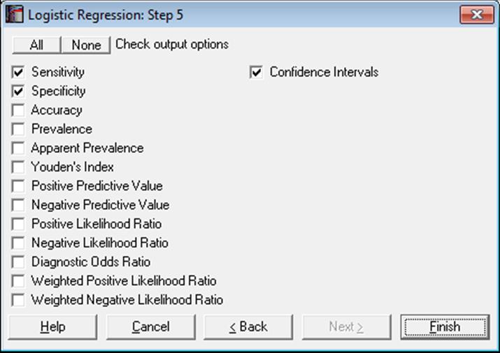
7.2.6.4. Logistic Regression Output Options
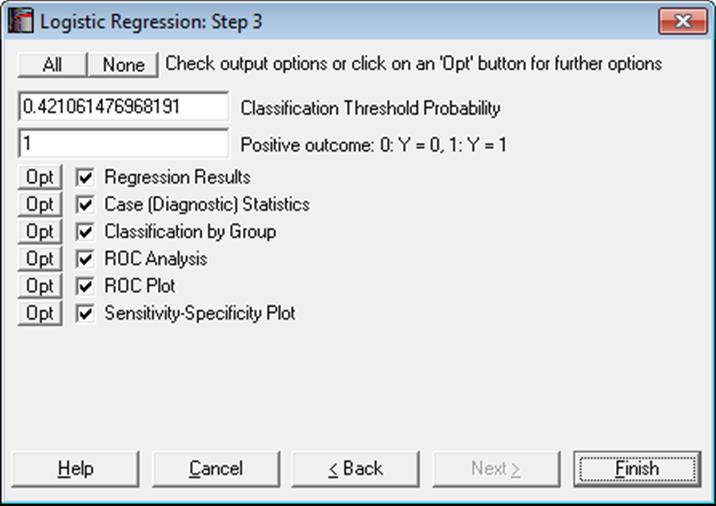
The Sensitivity-Specificity Plot option will not be available when Run a separate regression for each independent variable option is selected in the Intermediate Inputs dialogue.
Classification Threshold Probability: As described above for ROC Optimality Criterion, the estimated Classification threshold probability can be edited to try different scenarios. Changing this value will affect the output in Classification by Group and the Predicted Group and misclassifications in the Case (Diagnostic) Statistics output.
Positive Outcome: When calculating the Statistics For Diagnostic Tests output (e.g. sensitivity, specificity), UNISTAT assumes that the positive outcome is represented by 1 in the dependent variable and the true positive outcome of the test is represented in cell (1,1) of the 2 x 2 Table. Here you can control which value of the dependent variables represents the positive outcome, without affecting the rest of the Logistic Regression output.
Multicollinearity: Variables causing multicollinearity will be displayed with a zero coefficient at the end of the coefficients table. If you do not wish to display these variables enter the following line in the [Options] section of Documents\Unistat10\Unistat10.ini file:
DispCollin=0
The rest of the coefficients will be determined as if the regression were run without the variables causing collinearity.
7.2.6.4.1. Logistic Regression Results
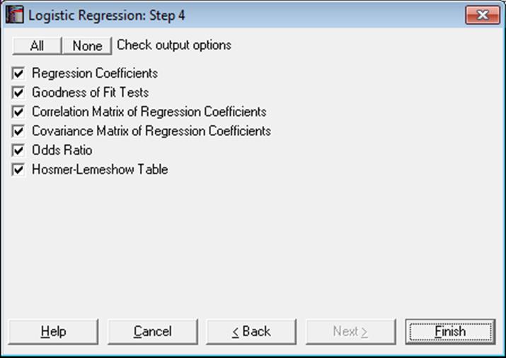
The main regression output displays a table for coefficients of the estimated regression equation, their standard errors, Wald statistics, probability values and confidence intervals for the significance level specified in the Variable Selection Dialogue. If any independent variables have been omitted due to multicollinearity, they are reported at the end of the table with a zero coefficient.
Regression Coefficients:
The Wald statistic is defined as:
![]()
and has a chi-square distribution with one degree of freedom.
The confidence intervals for regression coefficients are computed from:
![]()
where each coefficient’s standard error, ![]() , is the square root of the diagonal
element of the covariance matrix.
, is the square root of the diagonal
element of the covariance matrix.
Goodness of Fit Tests:
-2 Log-Likelihood for Initial Model (Null Deviance): This is -2 times the value when all independent variables are excluded from the model:
![]()
-2 Log-Likelihood for Final Model (Deviance): This is -2 times the value of the log likelihood function when convergence is achieved.
Likelihood Ratio: This is a test statistic for the null hypothesis that “all regression coefficients for covariates are zero”. It is equal to -2 times the difference between the initial and final model likelihood values and has a chi-square distribution with k degrees of freedom (the number of independent variables in the model).
Pearson: This is is for the observed versus expected number of responses. It has a chi-square distribution with n – k degrees of freedom (the number of valid cases minus the number of independent variables, including the constant term, if any).
![]()
Hosmer-Lemeshow Test: This is a test for lack of fit. The observations are sorted according to their fitted Y values (estimated probabilities) in ascending order. The identical cases of independent variables are formed into blocks. Then the cases are grouped into approximately ten classes without splitting the blocks.
The test statistic is defined as:
![]()
with g – 2 degrees of freedom, where:
g is the number of classes,
nj is the number of observations in the jth class,
Oj is the observed number of cases in the jth class,
Ej is the expected number of cases in the jth class.
Pseudo R-squared: In Logistic Regression (as well as in other maximum likelihood procedures), an R-squared statistic as in Linear Regression is not available. This is because Logistic Regression employs an iterative maximum likelihood estimation method. Equivalent statistics to test the goodness of fit have been proposed using the initial (L0) and maximum (L1) likelihood values.
McFadden:
![]()
Adjusted McFadden:
![]()
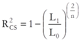
Cox & Snell:
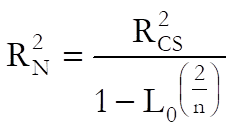
Nagelkerke:
Correlation Matrix of Regression Coefficients: This is a symmetric matrix with unity diagonal elements. The off-diagonal elements give correlations between regression coefficients.
Covariance Matrix of Regression Coefficients: This is a symmetric matrix where the square roots of the diagonal elements are the parameter standard errors. The off-diagonal elements are covariances between the regression coefficients.
Odds Ratio: Values of the odds ratio indicate the influence of one unit change in a covariate on the regression. It is defined as:
![]()
The standard error of the odds ratio is found as:
![]()
where![]() is the ith
coefficient’s standard error, and its confidence intervals as:
is the ith
coefficient’s standard error, and its confidence intervals as:
![]()
which are simply the exponential of the coefficient confidence intervals.
Hosmer-Lemeshow Table: The contingency table described above in Hosmer-Lemeshow Test is displayed. The observed and expected values for both values of the independent variable are listed for all classes.
7.2.6.4.2. Logistic Regression Case (Diagnostic) Statistics
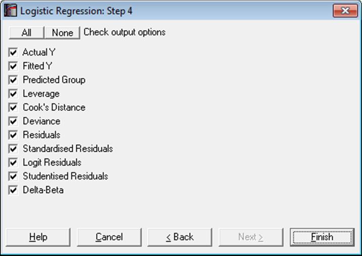
Case statistics are useful to determine the influence of individual observations on the overall fit of the model. For further information see 7.2.1.2.2. Linear Regression Case Output.
Predictions (Interpolations): There are three conditions under which predictions will be computed for estimated Y values:
1) If, for a case, all independent variables are non-missing, but only the dependent variable is missing,
2) if a case does not contain missing values but it has been omitted from the analysis by Data Processor’s Data → Select Row function and
3) if a case does not contain missing values but it has been omitted from the analysis by selecting subsamples from the Variable Selection Dialogue (see 2.1.2. Categorical Data Analysis).
Such cases are not included in the estimation of the model. When, however, Case (Diagnostic) Statistics option is selected, the program will detect these cases and compute and display the fitted (estimated) Y values, as well as their confidence intervals and some other related statistics. Therefore, it will be a good idea to include the cases for which predictions are to be made in the data matrix during the data preparation phase, and then exclude them from the analysis by one of the above three methods. When a case is predicted, its label will be prefixed by an asterisk (*).
In Stand-Alone Mode, the spreadsheet function Reg can also be used to make predictions (see 3.4.2.6.3. UNISTAT Functions).
This will give the logit of predicted values, which can be transformed back as:
![]()
Statistics available under Case (Diagnostic) Statistics option are as follows.
Case Labels: If row labels exist in data, they are displayed as case labels. Otherwise the row numbers are displayed. If a fitted Y value is predicted (see Fitted Y Values below) its label is marked by an asterisk (*). The misclassified cases (i.e. where an actual Y value differs from a predicted group) are divided into two groups as False Positive and False Negative and are marked by F+ and F- respectively.
Actual Y: Encoded values of the dependent variable (yi) are displayed.
Fitted Y: These are the estimated values for the dependent variable.
![]()
where:
![]()
If, for a case, all dependent variables are nonmissing, but the dependent variable is missing, the fitted (i.e. predicted) Y value will be displayed (see 7.2.6. Logistic Regression). Such cases are marked by a single asterisk (*) in their label.
Predicted Group: If ![]() cut-off (classification threshold) probability, then the group is 1, and 0 otherwise.
cut-off (classification threshold) probability, then the group is 1, and 0 otherwise.
Leverage:
![]()
where the vector:
![]()
Cook’s Distance:
![]()
where ![]() is
the standardised residual as defined below.
is
the standardised residual as defined below.
Deviance:
![]() if
if
![]() and
and ![]() otherwise, where:
otherwise, where:
![]()
Residuals:
![]()
Standardised Residuals:
![]()
Logit Residuals:
![]()
Studentised Residuals:
![]()
Delta-Beta:
![]()
Delta-beta is defined as the change in an estimated coefficient when a case is omitted from the analysis. An estimate can be computed from the above formula without having to run n regressions.
7.2.6.4.3. Classification by Group
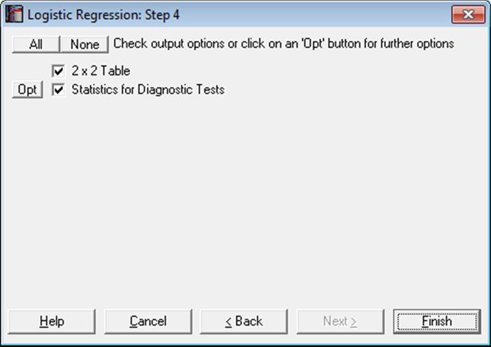
2 x 2 Table: The observed group membership (the actual Y in terms of 0 and 1) is tabulated against the estimated group membership. By default, it is assumed that the dependent variable value 1 represents the positive outcome The estimated group membership is 1 for any case with an estimated probability (fitted Y value) greater than or equal to the Classification Threshold Probability and it is 0 otherwise. If 1 does not represent the positive outcome of the test, then you can change this by entering 0 in the Positive Outcome box on the Output Options Dialogue. This will not force a re-estimation of the model.
|
|
Positive Actual |
Negative Actual |
Total |
|
Positive Estimate |
TP |
FP |
TP + FP |
|
Negative Estimate |
FN |
TN |
FN + TN |
|
Total |
TP + FN |
FP + TN |
TOTAL |
The table entries are defined as:
TP: True Positive: Correct acceptance,
TN: True Negative: Correct rejection,
FP: False Positive: False alarm (Type I error),
FN: False Negative: Missed detection (Type II error).
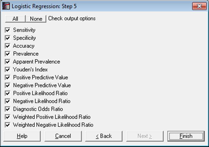
Statistics for Diagnostic Tests: These are the tests to determine how good a diagnostic method is, for instance, in detecting a positive outcome (i.e. sensitivity) or a negative outcome (i.e. specificity). Many of the statistics displayed here are proportions and their confidence intervals are computed employing the Wald (asymptotic) and Clopper-Pearson (exact) methods for binomial proportions (see 6.4.3.2. Binomial Test). Confidence intervals for likelihood ratios are computed as in Simel D., Samsa G., Matchar D. (1991).
The tests covered under this topic are also available in other procedures. When the data consists of two binary variables Actual and Estimate, you can use the Paired Proportions (see 6.4.5.6. Statistics for Diagnostic Tests) or Cross-Tabulation procedures. Alternatively, when you have an already formed 2 x 2 table, you can use the Contingency Table procedure.
Sensitivity: True positive rate or the probability of diagnosing a case as positive when it is actually positive.
TP / (TP + FN)
Specificity: True negative rate or the probability of diagnosing a case as negative when it is actually negative.
TN / (TN + FP)
Accuracy: The rate of correctly classified or the probability of true positive results, including true positive and true negative.
Sensitivity * Prevalence + Specificity * (1 – Prevalence)
(TP + TN) / TOTAL
Prevalence: The actual positive rate.
(TP + FN) / TOTAL
Apparent Prevalence: The estimated positive rate.
(TP + FP) / TOTAL
Youden’s Index: Confidence intervals are calculated as in Bangdiwala S.I., Haedo A.S., Natal M.L. (2008).
Sensitivity + Specificity
TP / (TP + FN) + TN / (FP + TN)
Positive Predictive Value: PPV
TP / (TP + FP)
Negative Predictive Value: NPV
TN / (FN + TN)
Positive Likelihood Ratio: LR+
Sensitivity / (1 – Specificity)
(TP / (TP + FN)) / (1 – (TN / (FP + TN)))
Negative Likelihood Ratio: LR-
(1 – Sensitivity) / Specificity
(1 – (TP / (TP + FN))) / (TN / (FP + TN))
Diagnostic Odds Ratio: Confidence intervals are calculated as in Scott I.A., Greenburg P.B., Poole P.J. (2008).
Positive Likelihood Ratio / Negative Likelihood Ratio
(TP * TN) / (FP * FN)
Weighted Positive Likelihood Ratio: WLR+. LR+ is weighted by prevalence.
(Prevalence * Sensitivity) / ((1-Prevalence)(1-Specificity))
TP / FP
Weighted Negative Likelihood Ratio: WLR-. LR- is weighted by prevalence.
(Prevalence (1-Sensitivity)) / ((1-Prevalence) Specificity)
FN / TN
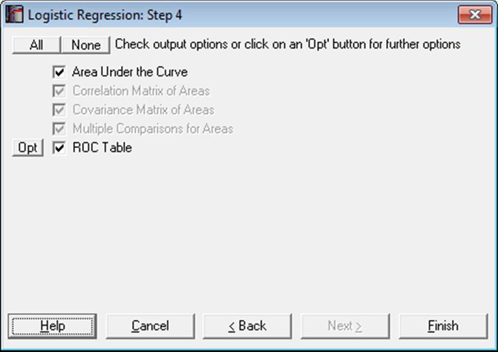
7.2.6.4.4. ROC Analysis
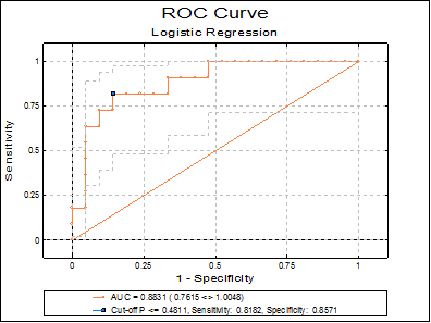
ROC analysis is widely used in assessing the statistical significance of diagnostic laboratory tests. Sensitivity and specificity values are computed for all fitted Y values. The best cut-off point is determined according to the ROC Optimality Criterion selected in the Intermediate Inputs dialogue. This can be Maximum sum of sensitivity and specificity (i.e. the Youden’s index) or the value nearest to the top-left corner of ROC curve. The ROC curve is obtained by plotting the sensitivity values against 1 – specificity.
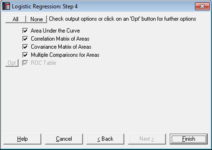
The output options for multiple ROC curves will not be available unless the Run a separate regression for each independent variable option is selected in the Intermediate Inputs dialogue.
Area Under the Curve (AUC): The area enclosed under the ROC curve is calculated by employing the algorithm developed by Delong E.R., Delong D.M., Clarke-Pearson D.L. (1998), which is based on the Mann-Whitney U test statistic. This not only produces an identical result to the area calculated by the trapezoidal rule, but also provides the standard errors (covariances) necessary to statistically compare AUCs, based on the nonparametric U-distribution (see 6.4.1.1. Mann-Whitney U Test).
AUC is a measure of the predictive power of the model. A value of 0.5 (which means that the curve is a 45º line) shows that the model has no power. A value of 1 (the theoretical maximum) means the full, 100% explanatory power.
The output includes AUCs, their standard errors, tail probabilities and the confidence intervals (asymptotic normal).
Correlation and Covariance Matrices for Areas: These options are available only when the Run a separate regression for each independent variable option is selected in the Intermediate Inputs dialogue.
Multiple Comparisons for Areas: This option is available only when the Run a separate regression for each independent variable option is selected in the Intermediate Inputs dialogue. The difference between all possible pairs of AUCs, their standard errors and confidence intervals are displayed.
The output includes the difference between AUCs, their standard errors, tail probabilities and confidence intervals (asymptotic normal) and a further chi-square test with 1 degree of freedom.
ROC Table: All Statistics for Diagnostic Tests and their confidence intervals are computed for all fitted Y values (classification threshold probabilities). By default, only the sensitivity and specificity values and their confidence intervals are displayed. However, the user can choose to display any statistic with or without confidence intervals. The case (row) corresponding to the Classification Threshold Probability (the best cut-off point) is marked by an asterisk.
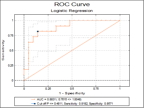
7.2.6.4.5. Receiver Operating Characteristic (ROC) Plot
Sensitivity and specificity values are computed for all classification threshold (cut-off) probabilities. For each probability, the sensitivity value is plotted against 1 – specificity. The best cut-off point is marked by a symbol on the curve.
When only one ROC curve is plotted, its confidence intervals are also displayed on the graph. The AUC, its confidence interval, sensitivity and specificity values are displayed in the legend. If there is only one independent variable, then its value corresponding to the best cut-off point is also displayed. When there are multiple independent variables, the best cut-off probability is displayed instead. The display of confidence intervals can be switch on or off from Edit → Data Series dialogue.
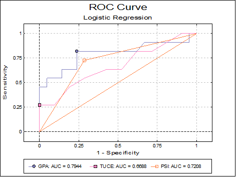
If the Run a separate regression for each independent variable option is selected in the Intermediate Inputs dialogue (i.e. if multiple ROCs are compared), the ROC plot is not output for each independent variable separately. In this case only one plot is drawn at the end of the output, with multiple ROC curves and without confidence intervals. For each curve, the area enclosed under the curve (AUC) is displayed in the legend. The best cut-off point is also marked by a symbol on each curve.
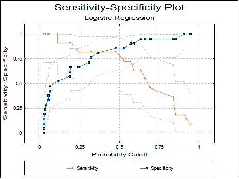
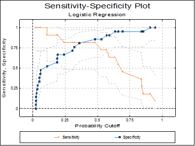
7.2.6.4.6. Sensitivitiy-Specificity Plot
This plot is similar to the ROC plot, except that sensitivity and specificity values are plotted against all values of the classification probability. This plot is not available when the Run a separate regression for each independent variable option is selected in the Intermediate Inputs dialogue.
7.2.6.5. Logistic Regression Examples
Example 1
Open LOGIT and select Statistics 1 → Regression Analysis → Logistic Regression. From the Variable Selection Dialogue select GPA, TUCE and PSI (C12 to C14) as [Variable]s and GRADE (C15) as [Dependent] and. On the Intermediate Inputs dialogue select the Run regression with all independent variables option.
Some of the following results have been shortened to save space.
Logistic Regression
Dependent Variable: GRADE
Minimum of dependent variable is encoded as 0 and the rest as 1.
Valid Number of Cases: 32, 0 Omitted
Regression Coefficients
|
|
Coefficient |
Standard Error |
Wald Statistic |
Probability |
Lower 95% |
Upper 95% |
|
Constant |
-13.0213 |
4.9313 |
6.9724 |
0.0083 |
-22.6866 |
-3.3561 |
|
GPA |
2.8261 |
1.2629 |
5.0074 |
0.0252 |
0.3508 |
5.3014 |
|
TUCE |
0.0952 |
0.1416 |
0.4519 |
0.5014 |
-0.1823 |
0.3726 |
|
PSI |
2.3787 |
1.0646 |
4.9926 |
0.0255 |
0.2922 |
4.4652 |
Goodness of Fit Tests
|
|
-2 Log likelihood |
|
Initial Model |
41.1835 |
|
Final Model |
25.7793 |
|
|
Chi-Square Statistic |
Degrees of Freedom |
Right-Tail Probability |
|
Pearson |
27.2571 |
28 |
0.5043 |
|
Null Deviance |
41.1835 |
31 |
0.1045 |
|
Deviance |
25.7793 |
28 |
0.5852 |
|
Likelihood Ratio |
15.4042 |
3 |
0.0015 |
|
Hosmer-Lemeshow |
7.4526 |
8 |
0.4887 |
|
|
Pseudo R-squared |
|
McFadden |
0.3740 |
|
Adjusted McFadden |
0.1798 |
|
Cox & Snell |
0.3821 |
|
Nagelkerke |
0.5278 |
Correlation Matrix of Regression Coefficients
|
|
Constant |
GPA |
TUCE |
PSI |
|
Constant |
1.0000 |
-0.7343 |
-0.4960 |
-0.4494 |
|
GPA |
-0.7343 |
1.0000 |
-0.2065 |
0.3181 |
|
TUCE |
-0.4960 |
-0.2065 |
1.0000 |
0.0990 |
|
PSI |
-0.4494 |
0.3181 |
0.0990 |
1.0000 |
Covariance Matrix of Regression Coefficients
|
|
Constant |
GPA |
TUCE |
PSI |
|
Constant |
24.3180 |
-4.5735 |
-0.3463 |
-2.3592 |
|
GPA |
-4.5735 |
1.5950 |
-0.0369 |
0.4276 |
|
TUCE |
-0.3463 |
-0.0369 |
0.0200 |
0.0149 |
|
PSI |
-2.3592 |
0.4276 |
0.0149 |
1.1333 |
Odds Ratio
|
|
Odds Ratio |
Standard Error |
Lower 95% |
Upper 95% |
|
GPA |
16.8797 |
21.3181 |
1.4202 |
200.6239 |
|
TUCE |
1.0998 |
0.1557 |
0.8334 |
1.4515 |
|
PSI |
10.7907 |
11.4874 |
1.3393 |
86.9380 |
Hosmer-Lemeshow Table
|
|
Actual Y = 0 |
Expected Y = 0 |
Actual Y = 1 |
Expected Y = 1 |
Total |
|
1 |
4 |
3.8965 |
0 |
0.1035 |
4 |
|
2 |
3 |
2.8964 |
0 |
0.1036 |
3 |
|
3 |
3 |
2.8353 |
0 |
0.1647 |
3 |
|
4 |
2 |
2.7165 |
1 |
0.2835 |
3 |
|
5 |
2 |
2.4295 |
1 |
0.5705 |
3 |
|
6 |
4 |
2.7678 |
0 |
1.2322 |
4 |
|
7 |
1 |
1.4199 |
2 |
1.5801 |
3 |
|
8 |
1 |
1.1139 |
2 |
1.8861 |
3 |
|
9 |
0 |
0.6265 |
3 |
2.3735 |
3 |
|
10 |
1 |
0.2977 |
2 |
2.7023 |
3 |
Case (Diagnostic) Statistics
|
|
Actual Y |
Fitted Y |
Predicted Group |
Leverage |
Cook’s Distance |
Deviance |
|
1 |
0.0000 |
0.0266 |
0.0000 |
0.0390 |
0.0011 |
-0.2321 |
|
2 |
0.0000 |
0.0595 |
0.0000 |
0.0545 |
0.0036 |
-0.3503 |
|
3 |
0.0000 |
0.1873 |
0.0000 |
0.0889 |
0.0225 |
-0.6440 |
|
… |
… |
… |
… |
… |
… |
… |
|
30 |
1.0000 |
0.9453 |
1.0000 |
0.0853 |
0.0054 |
0.3353 |
|
F+ 31 |
0.0000 |
0.5291 |
1.0000 |
0.1171 |
0.1490 |
-1.2273 |
|
F- 32 |
1.0000 |
0.1110 |
0.0000 |
0.1299 |
1.1953 |
2.0966 |
|
|
Residuals |
Standardised Residuals |
Logit Residuals |
Studentised Residuals |
|
1 |
-0.0266 |
-0.1652 |
-1.0273 |
-0.2368 |
|
2 |
-0.0595 |
-0.2515 |
-1.0633 |
-0.3602 |
|
3 |
-0.1873 |
-0.4800 |
-1.2304 |
-0.6747 |
|
… |
… |
… |
… |
… |
|
30 |
0.0547 |
0.2405 |
1.0578 |
0.3506 |
|
F+ 31 |
-0.5291 |
-1.0600 |
-2.1237 |
-1.3061 |
|
F- 32 |
0.8890 |
2.8296 |
9.0065 |
2.2477 |
F+: False Positive
F-: False Negative
2 x 2 Table
|
Estimated \ Actual |
Positive |
Negative |
Total |
|
Positive |
9 |
3 |
12 |
|
|
81.82% |
14.29% |
|
|
Negative |
2 |
18 |
20 |
|
|
18.18% |
85.71% |
|
|
Total |
11 |
21 |
32 |
|
|
100.00% |
100.00% |
|
|
Classification Threshold Probability = |
0.4211 |
Statistics for Diagnostic Tests
Confidence Intervals: Row 1: Asymptotic Normal, Row 2: Exact Binomial
|
|
Value |
Standard Error |
Lower 95% |
Upper 95% |
|
Sensitivity |
0.8182 |
0.1163 |
0.5903 |
1.0000 |
|
|
|
|
0.4822 |
0.9772 |
|
Specificity |
0.8571 |
0.0764 |
0.7075 |
1.0000 |
|
|
|
|
0.6366 |
0.9695 |
|
Accuracy |
0.8438 |
0.0642 |
0.7179 |
0.9696 |
|
|
|
|
0.6721 |
0.9472 |
|
Prevalence |
0.3438 |
0.0840 |
0.1792 |
0.5083 |
|
|
|
|
0.1857 |
0.5319 |
|
Apparent Prevalence |
0.3750 |
0.0856 |
0.2073 |
0.5427 |
|
|
|
|
0.2110 |
0.5631 |
|
Youden’s Index |
0.6753 |
|
|
|
|
|
|
|
0.1188 |
0.9467 |
|
Positive Predictive Value |
0.7500 |
0.1250 |
0.5050 |
0.9950 |
|
|
|
|
0.4281 |
0.9451 |
|
Negative Predictive Value |
0.9000 |
0.0671 |
0.7685 |
1.0000 |
|
|
|
|
0.6830 |
0.9877 |
|
Positive Likelihood Ratio |
5.7273 |
|
1.9371 |
16.9334 |
|
Negative Likelihood Ratio |
0.2121 |
|
0.0596 |
0.7547 |
|
Diagnostic Odds Ratio |
27.0000 |
|
3.8033 |
191.6750 |
|
Weighted Positive Likelihood Ratio |
3.0000 |
|
1.0678 |
8.4284 |
|
Weighted Negative Likelihood Ratio |
0.1111 |
|
0.0295 |
0.4183 |
Logistic Regression
Dependent Variable: GRADE
Minimum of dependent variable is encoded as 0 and the rest as 1.
Valid Number of Cases: 32, 0 Omitted
Area Under the Curve
|
|
AUC |
Standard Error |
Z-Statistic |
1-Tail Probability |
2-Tail Probability |
Lower 95% |
Upper 95% |
|
|
0.8831 |
0.0621 |
6.1721 |
0.0000 |
0.0000 |
0.7615 |
1.0048 |
ROC Table
* marks the best cut-off case.
Optimality criterion: Max(Sensitivity + Specificity)
Confidence Intervals: Asymptotic Normal
|
|
Cut-off P <= |
Sensitivity |
Lower 95% |
Upper 95% |
Specificity |
Lower 95% |
Upper 95% |
|
1 |
0.9453 |
0.0909 |
0.0000 |
0.2608 |
1.0000 |
1.0000 |
1.0000 |
|
2 |
0.9048 |
0.1818 |
0.0000 |
0.4097 |
1.0000 |
1.0000 |
1.0000 |
|
3 |
0.8521 |
0.1818 |
0.0000 |
0.4097 |
0.9524 |
0.8613 |
1.0000 |
|
… |
… |
… |
… |
… |
… |
… |
… |
|
10 |
0.5699 |
0.7273 |
0.4641 |
0.9905 |
0.9048 |
0.7792 |
1.0000 |
|
11 |
0.5291 |
0.7273 |
0.4641 |
0.9905 |
0.8571 |
0.7075 |
1.0000 |
|
* 12 |
0.4811 |
0.8182 |
0.5903 |
1.0000 |
0.8571 |
0.7075 |
1.0000 |
|
… |
… |
… |
… |
… |
… |
… |
… |
|
30 |
0.0265 |
1.0000 |
1.0000 |
1.0000 |
0.0952 |
0.0000 |
0.2208 |
|
31 |
0.0259 |
1.0000 |
1.0000 |
1.0000 |
0.0476 |
0.0000 |
0.1387 |
|
32 |
0.0245 |
1.0000 |
1.0000 |
1.0000 |
0.0000 |
0.0000 |
0.0000 |
|
Range of best Classification Threshold Probability = |
0.3610 <> 0.4811 |
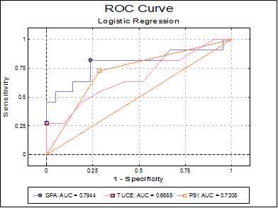
Example 2
Continuing from the above example, this time select the Run a separate regression for each independent variable option on the Intermediate Inputs dialogue. Also uncheck the first three output options Regression Results, Case (Diagnostic) Statistics and Classification by Group.
Logistic Regression
Dependent Variable: GRADE
Minimum of dependent variable is encoded as 0 and the rest as 1.
Valid Number of Cases: 32, 0 Omitted
Area Under the Curve
|
|
AUC |
Standard Error |
Z-Statistic |
1-Tail Prob |
2-Tail Prob |
Lower 95% |
Upper 95% |
|
GPA |
0.7944 |
0.1001 |
2.9421 |
0.0016 |
0.0033 |
0.5983 |
0.9905 |
|
TUCE |
0.6688 |
0.1075 |
1.5702 |
0.0582 |
0.1164 |
0.4581 |
0.8796 |
|
PSI |
0.7208 |
0.0867 |
2.5477 |
0.0054 |
0.0108 |
0.5509 |
0.8906 |
Correlation Matrix of Areas
|
|
GPA |
TUCE |
PSI |
|
GPA |
1.0000 |
0.2215 |
-0.2182 |
|
TUCE |
0.2215 |
1.0000 |
-0.0997 |
|
PSI |
-0.2182 |
-0.0997 |
1.0000 |
Covariance Matrix of Areas
|
|
GPA |
TUCE |
PSI |
|
GPA |
0.0100 |
0.0024 |
-0.0019 |
|
TUCE |
0.0024 |
0.0116 |
-0.0009 |
|
PSI |
-0.0019 |
-0.0009 |
0.0075 |
Multiple Comparisons for Areas
|
|
Difference |
Standard Error |
Z-Statistic |
1-Tail Probability |
2-Tail Probability |
|
GPA – TUCE |
0.1255 |
0.1296 |
0.9684 |
0.1664 |
0.3328 |
|
GPA – PSI |
0.0736 |
0.1460 |
0.5042 |
0.3071 |
0.6141 |
|
TUCE – PSI |
-0.0519 |
0.1447 |
0.3591 |
0.3598 |
0.7195 |
|
|
Lower 95% |
Upper 95% |
Chi-Square Statistic |
Right-Tail Probability |
|
GPA – TUCE |
-0.1285 |
0.3796 |
0.9378 |
0.3328 |
|
GPA – PSI |
-0.2125 |
0.3597 |
0.2542 |
0.6141 |
|
TUCE – PSI |
-0.3355 |
0.2316 |
0.1289 |
0.7195 |