6.6.1. Contingency Table
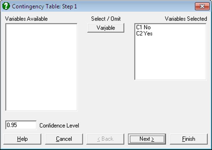
This procedure assumes that the data is in the form of frequency counts and entered in a table format. Any number of data columns can be selected as the columns of a Contingency Table, provided that their lengths are equal. If this condition is not met, then the program will not proceed.
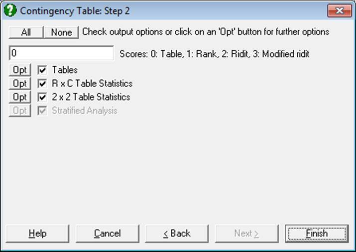
After selecting the variables, an Output Options Dialogue asking for the score method to be used (see 6.6.2.0. Scores) and containing four check boxes (with an [Opt] button to their left) will be displayed. Each one of these options has further options. The full output from the Contingency Table procedure is large and computations are demanding. For a full discussion of these options see section 6.6.2. Cross-Tabulation.
Example 1
Example 23.1 on p. 490 from Zar, J. H. (2010). The null hypothesis “Human hair colour is independent of sex in the population sampled” is tested.
Open TABLES, select Statistics 1 → Tables → Contingency Table and select Black, Brown, Blond and Red (C1 to C4) as [Variable]s. From the Tables options select only the Frequency and from R x C Table Statistics select only the Chi-square Tests output options. Go back to Step 2 Output Options Dialogue and click [Finish] to obtain the following results:
Contingency Table
2 Rows x 4 Columns
Frequency
|
|
Black |
Brown |
Blond |
Red |
Row Sum |
|
R1 |
32.0000 |
43.0000 |
16.0000 |
9.0000 |
100.0000 |
|
R2 |
55.0000 |
65.0000 |
64.0000 |
16.0000 |
200.0000 |
|
Column Sum |
87.0000 |
108.0000 |
80.0000 |
25.0000 |
300.0000 |
Chi-square Tests
|
|
Chi-Square Statistic |
Degrees of Freedom |
Right-Tail Probability |
|
Pearson |
8.9872 |
3 |
0.0295 |
|
Likelihood-Ratio |
9.5121 |
3 |
0.0232 |
|
+ Yates Correction |
|
|
|
|
# Linear-by-linear |
2.6155 |
1 |
0.1058 |
|
~ McNemar-Bowker |
|
|
|
+ Reported for 2 x 2 tables.
# Table scores
~ Reported for 3 x 3 or larger square tables.
Cells with expected count < 5 = 0 ( 0.00%)
Minimum expected count = 8.3333
|
Phi = |
0.1731 |
|
Contingency Coefficient = |
0.1705 |
|
Cramer’s V = |
0.1731 |
In this example Zar only reports Pearson’s chi-square statistic and its tail probability.
Example 2
Example 23.4 on p. 499 from Zar, J. H. (2010). The null hypothesis “the ability of snails to resist the current is no different between the two species” is tested. Open TABLES, select Statistics 1 → Tables → Contingency Table, select Resisted and Yielded (C10 and C11) as [Variable]s. Leave output option selections as in the previous example.
Contingency Table
2 Rows x 2 Columns
Frequency
|
|
Resisted |
Yielded |
Row Sum |
|
R1 |
12.0000 |
7.0000 |
19.0000 |
|
R2 |
2.0000 |
9.0000 |
11.0000 |
|
Column Sum |
14.0000 |
16.0000 |
30.0000 |
Chi-square Tests
|
|
Chi-Square Statistic |
Degrees of Freedom |
Right-Tail Probability |
|
Pearson |
5.6622 |
1 |
0.0173 |
|
Likelihood-Ratio |
6.0162 |
1 |
0.0142 |
|
+ Yates Correction |
3.9993 |
1 |
0.0455 |
|
# Linear-by-linear |
5.4734 |
1 |
0.0193 |
|
~ McNemar-Bowker |
|
|
|
# Table scores
~ Reported for 3 x 3 or larger square tables.
Cells with expected count < 5 = 0 ( 0.00%)
Minimum expected count = 5.1333
|
Phi = |
0.4344 |
|
Contingency Coefficient = |
0.3985 |
|
Cramer’s V = |
0.4344 |
Zar reports the chi-square statistic with Yates correction and its tail probability.
Example 3
Example 8.4 on p. 231 from Armitage & Berry (2002). The effects of PAS and streptomycin in the treatment of pulmonary tuberculosis are given. The null hypothesis “the probabilities for rows (columns) to fall into different columns (rows) are the same” is tested.
Open TABLES, select Statistics 1 → Tables → Contingency Table and include Negative smear, NegSmr-PosCult and NegSmr-NegCult (C7 to C9) as [Variable]s. Include only Frequency, Expected and Chi-square Statistics output options to obtain the following results:
Contingency Table
3 Rows x 3 Columns
Frequency
|
|
Negative smear |
NegSmr-PosCult |
NegSmr-NegCult |
Row Sum |
|
R1 |
56.0000 |
30.0000 |
13.0000 |
99.0000 |
|
R2 |
46.0000 |
18.0000 |
20.0000 |
84.0000 |
|
R3 |
37.0000 |
18.0000 |
35.0000 |
90.0000 |
|
Column Sum |
139.0000 |
66.0000 |
68.0000 |
273.0000 |
Expected
|
|
Negative smear |
NegSmr-PosCult |
NegSmr-NegCult |
|
R1 |
50.4066 |
23.9341 |
24.6593 |
|
R2 |
42.7692 |
20.3077 |
20.9231 |
|
R3 |
45.8242 |
21.7582 |
22.4176 |
Chi-square Tests
|
|
Chi-Square Statistic |
Degrees of Freedom |
Right-Tail Probability |
|
Pearson |
17.6284 |
4 |
0.0015 |
|
Likelihood-Ratio |
17.7770 |
4 |
0.0014 |
|
+ Yates Correction |
|
|
|
|
# Linear-by-linear |
11.4263 |
1 |
0.0007 |
|
McNemar-Bowker |
14.9937 |
3 |
0.0018 |
+ Reported for 2 x 2 tables.
# Table scores
Cells with expected count < 5 = 0 ( 0.00%)
Minimum expected count = 20.3077
|
Phi = |
0.2541 |
|
Contingency Coefficient = |
0.2463 |
|
Cramer’s V = |
0.1797 |