6.6.2. Cross-Tabulation

Multi-way cross-tabulations with or without weights can be performed.

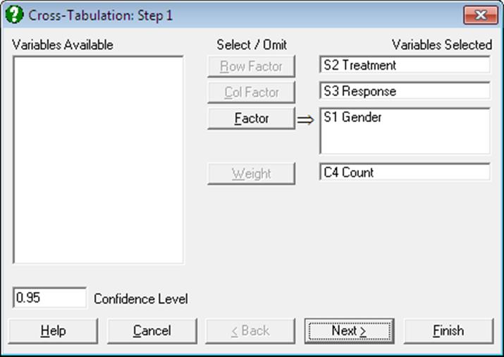
At least one factor column should be assigned as the [Row Factor] and another as the [Column Factor], whose categories are to be displayed on the rows and columns of the generated table respectively. Optionally, an unlimited number of further factor columns can be selected to run multi-way analyses. In this case, a further set of output options for Stratified Analysis will become available.

The program will sort each column separately, determine the number of categories in each and then count the frequency of occurrence of every combination of categories. For instance, in a two-way analysis, if the variable [Row Factor] takes on values 0, 1, and 2 and the variable [Column Factor] takes on four different values such as 3, 4, 5 and 6, the program will produce a 3 by 4 table (number of rows by number of a separate table and its associated statistics will be generated for each combination of factor levels selected.

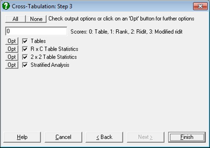
After processing the data, the program will prompt for output options. Note that not all output options will be available for all data sets. For instance, 2 x 2 Table Statistics option will be available when row and column factors have two levels each, and the Stratified Analysis option will only be available for Cross-Tabulation procedure when a factor column is selected.

6.6.2.0. Scores

Some of the statistics computed for this procedure depend on the ordering of rows and columns of the contingency table. These statistics are Linear-by-linear (also known as Mantel-Haenszel chi-square test), Pearson correlation, Eta and Cochran-Armitage trend test. First define the notation used in this section:

      n - sum total of all frequencies

      r - number of rows in contingency table

      c - number of columns in contingency table

      ri - sum of frequencies in the i^th row

      cj - sum of frequencies in the j^th column

One of the following four methods can be used:

Table scores: This is the default score method. The column and row index numbers are used as factor levels.

Rank scores: These are the rank values as used in Spearman rank correlation coefficient and they are computed as:

Ridit scores: These are the rank scores divided by the total sample size:

Modified ridit scores: These are the rank scores divided by the total sample size + 1:

6.6.2.1. Tables

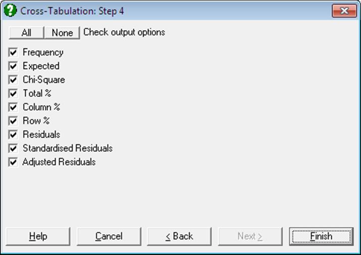
Each output option is displayed as a separate table, which can be sent to Data Processor for further analysis.

Frequency: For Contingency Table, this is the data as it exists in the spreadsheet. It may contain non-integer and / or missing data. For Cross-Tabulation, it consists of the computed frequency figures for categories represented by the row and column factors. Therefore, it always contains integers and no missing data. Define:

      This table also displays the row sum and column sum values on the table margins.

Expected Frequency: For each cell, the expected frequency is calculated as:

Chi-square: The contribution of each cell to the overall chi-square value is calculated as:

Total Percent: Percentage of the cell frequency out of sum total of all table frequencies:

      This table also displays the row sum (i.e. percentage of the row total out of sum total) and column sum (i.e. percentage of the column total out of sum total) percentages on the table margins.

Row Percent: Percentage of the cell frequency out of sum of frequencies in the same row.

Column Percent: Percentage of the cell frequency out of sum of frequencies in the same column.

Residual: Difference between observed and expected frequencies.

Standardised Residual:

Adjusted Residual:

6.6.2.2. R x C Table Statistics

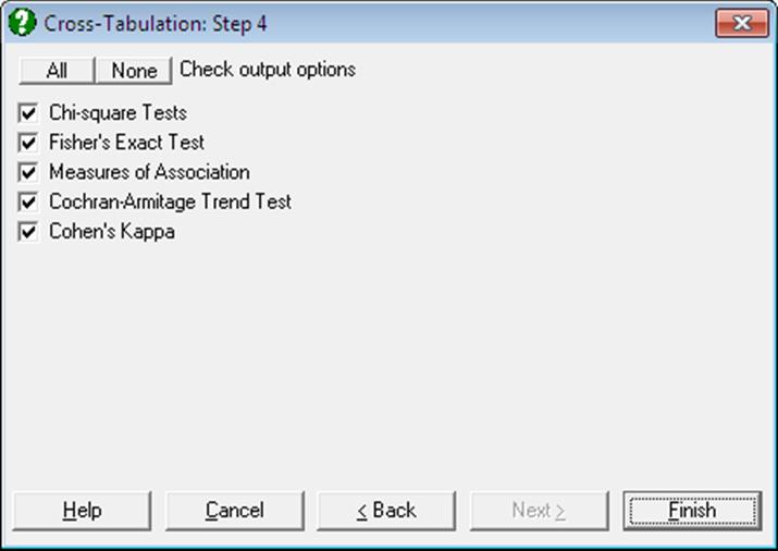
6.6.2.2.1. Chi-square Tests

Several chi-square significance tests and chi-square related coefficients are reported. The program also reports the number of cells with an expected frequency less than 5, its percentage out of total frequency and the minimum expected frequency. The aim of this information is to enable the user to judge whether the asymptotic probabilities reported here are reliable enough, or the exact probabilities like Fisher’s should be used.

Pearson Chi-square: This provides a measure of association between row and column factors.

     

     

      For rows and columns containing 0s only, the degrees of freedom is adjusted accordingly.

Likelihood Ratio: This involves the ratio of observed and expected frequencies.

     

     

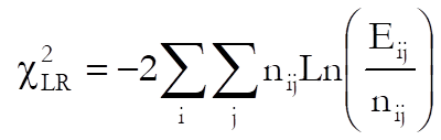
Yates Correction: Also known as continuity correction, this is reported for 2 x 2 tables only.

     

     

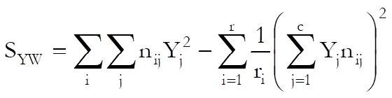
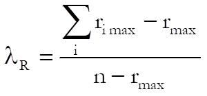
Linear-by-linear: This is also known as Mantel-Haenszel chi-square test. It tests the linear association between row and column factors:

     

     

      where R-squared is the Pearson correlation between the row factor and the column factor. The value of this test depends on the score method selected (see Scores).

McNemar-Bowker: This is a test of symmetry for square tables. Since it is identical to McNemar Test for 2 x 2 tables, it is reported only for 3 x 3 or larger square tables.

     

     

Phi Coefficient: For tables other than 2 x 2:

     

      and for 2 x 2 tables:

     

      with a magnitude equal to Pearson correlation coefficient R (see Linear-by-linear Test above). Note that phi coefficient for 2 x 2 tables can be negative.

Contingency Coefficient:

     

      where:

     

Cramer’s V Coefficient: For tables other than 2 x 2:

     

      and for 2 x 2 tables:

     

      Therefore, Cramer’s V coefficient for 2 x 2 tables can be negative.

6.6.2.2.2. Fisher’s Exact Test

Fisher’s Exact Test for R x C Tables is also known as the Freeman-Halton test. The network algorithm developed by Mehta and Patel (1983) is used to calculate the two-tailed and table probabilities. This procedure is computationally demanding and it may not be feasible for large tables. For 2 x 2 tables the results are identical to that of Fisher’s Exact Test which is available under the Paired Proportions procedure (see 6.6.2.3. 2 x 2 Table Statistics below. The latter procedure also reports the left- and right- tail probabilities in addition to two-tailed and table probabilities.

6.6.2.2.3. Measures of Association

Tests in this section are used to assess the association between row and column factors of the table. All test statistics (with the exception of eta) are reported with their standard errors and asymptotic confidence intervals using the standard normal distribution:

     

The first group of tests (Somer’s delta, Goodman-Kruskal’s gamma, Kendall’s tau b and tau c) will rank observations as concordant or discordant. Each observation is checked pairwise with all other observations to see whether its relative ordering is the same in the sequence. The ordering is called concordant if it is the same and discordant if it is different. Note that these tests are computationally demanding. If the table is large, they may take a long time to compute.

The following entities are computed:

·        C = number of concordant pairs

·        D = number of discordant pairs

·        Tx = number of ties in columns

·        Ty = number of ties in rows.

Goodman-Kruskall’s Gamma: This coefficient does not make an adjustment for ties. It is defined as:

     

      The value of gamma can be taken as the probability of correctly guessing the order of a pair of cases on one variable once the ordering on the other variable is known.

Kendall’s tau b: This statistic reflects the effect of ties both in columns and rows:

     

Kendall’s tau c: This is also called Stuart’s tau c.

     

      where T is sum total of all ranks and m is the minimum of number of columns or number of rows.

     

Pearson Correlation: The value of this test depends on the score method selected (see Scores).

     

      where:

     

     

     

Spearman Rank Correlation: The only difference from Pearson correlation is that ranks of factor levels (rank scores) are always used.

     

Eta: The value of this statistic depends on the score method selected (see Scores). The asymmetric eta for the column factor is defined as:

     

      where Yj are the levels of column factor and:

     

      Eta for the row factor can be obtained by reversing the indices.

The third group of tests of association will calculate a row statistic (given the column factor), a column statistic (given the row factor) and a symmetric statistic. Here we will only define the statistic for the row factor. The column statistic can be obtained by reversing the indices.

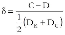
Somer’s Delta: Somer’s delta also uses concordant / discordant pairs to test asymmetric association between the row and column factors.

     

      where:

     

      and the symmetric delta is:

     

Goodman-Kruskall’s Lambda:

     

      where:

     

     

      and the symmetric lambda is the average of the two asymmetric lambdas:

     

Uncertainty Coefficient: This measures the proportion of uncertainty (entropy) in the column variable Y that is explained by the row variable X:

     

      where:

     

     

     

      and the symmetric uncertainty coefficient is:

     

6.6.2.2.4. Cochran-Armitage Trend Test

This test is available only for 2 x c or r x 2 tables. It provides a test statistic for the trend of binary proportions in levels of a factor with two or more levels (the response variable). The latter is assumed to contain binary responses (e.g. yes / no) and its levels are internally recoded as 0 and 1. For a table with two columns and r rows, the trend is defined as:

     

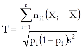
where:

     

and:

     

Here, is the i^th level of the row variable and is the weighted average of row variable levels. Therefore, Cochran-Armitage trend test depends on the score method selected (see Scores).

6.6.2.2.5. Cohen’s Kappa

Kappa is computed for square tables. Only an unweighted Kappa test is performed. For details see 6.5.10. Kappa Test for Inter-Observer Variation.

6.6.2.3. 2 x 2 Table Statistics

When a 2 x 2 table is formed, all statistics available under Binomial Proportion, Unpaired Proportions and Paired Proportions sections will also be available in this procedure. The user should take care to distinguish between the table formed by the Cross-Tabulation procedure and one formed on the same pair of columns by the Unpaired Proportions procedure. Here, the total table frequency is the number valid pairs (as in Paired Proportions), whereas in Unpaired Proportions the total frequency is the sum of valid cases in sample 1 and sample 2.

·      Binomial Test: This test is performed on the row factor and the column factor separately, i.e. on the row sums and the column sums of the table. Therefore, one needs to take this into consideration when the Contingency Table option is selected. By default, the program uses an expected proportion of 0.5. You can change this to any value between 0 and 1 from Binomial Proportion → Binomial Test procedure.

·      Noninferiority Test: This test is also performed on the row factor and the column factor separately. Expected proportion (default 0.5) and the noninferiority margin (default 0.2) can be changed from Binomial Proportion → Noninferiority Test procedure.

·      Superiority Test: This test is also performed on the row factor and the column factor separately. Expected proportion (default 0.5) and the superiority margin (default 0.2) can be changed from Binomial Proportion → Superiority Test procedure.

·      Equivalence Test for Binomial Proportion: This test is also performed on the row factor and the column factor separately. Expected proportion (default 0.5), the lower equivalence margin (default -0.2) and the upper equivalence margin (default 0.2) can be changed from Binomial Proportion → Equivalence Test for Binomial Proportion procedure.

·      Difference Between Unpaired Proportions

·      Risk Ratio

·      Odds Ratio and Relative Risks

·      Difference Between Paired Proportions

·      Fisher’s Exact Test

·      McNemar Test

·      Odds Ratio (Paired)

This facility is especially useful when the four frequency values for a 2 x 2 table are already available in the spreadsheet. In this case they will not have to be typed again into the Cell Frequencies are Given dialogue of the nonparametric tests.

6.6.2.4. Stratified Analysis

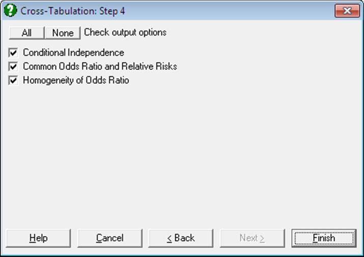
The tests in this group are available only for multi-way 2 x 2 cross-tabulations, i.e. when one or more factor variables are selected apart from the row and column factors, which have only two levels each. When a factor variable is selected, all tables and tests described above will be displayed once for each level (stratum) of the factor variable. The tests described in this section are reported only once at the end of the output.

6.6.2.4.1. Conditional Independence

These two chi-square statistics will test the independence of the row and column factors across strata.

Cochran:

     

     

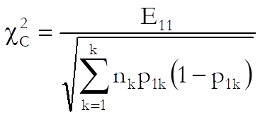
      where:

     

     

      and n_k is the total frequency of the k^th stratum.

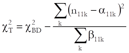
Mantel-Haenszel: This is similar to Cochran test but introduces a continuity correction:

     

     

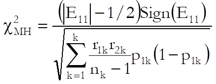
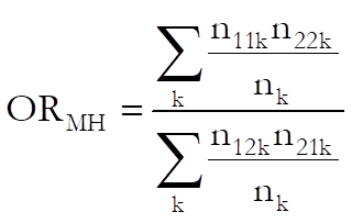
6.6.2.4.2. Common Odds Ratio and Relative Risks

The common odds ratio for multi-way 2 x 2 tables is estimated by Mantel-Haenszel and logit methods. The odds ratio for the k^th stratum is defined as:

    

See Odds Ratio and Relative Risks.

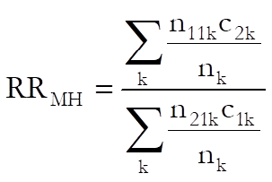
Mantel-Haenszel estimate: For multi-way tables the common odds ratio is defined as:

     

      and cohort 1 is:

     

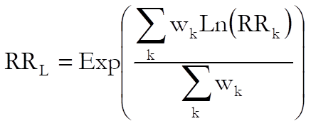
Logit estimate:

     

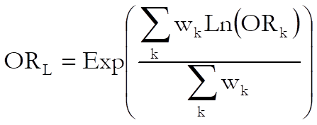
      where:

     

      and cohort 1 is:

     

6.6.2.4.3. Homogeneity of Odds Ratio

The null hypothesis “odds ratios across strata are equal” is tested.

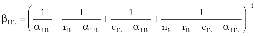
Breslow-Day: This test is based on Mantel-Haenszel estimate of the common odds ratio:

     

     

      where:

     

     

Tarone: This is a modification of Breslow-Day test:

     

     

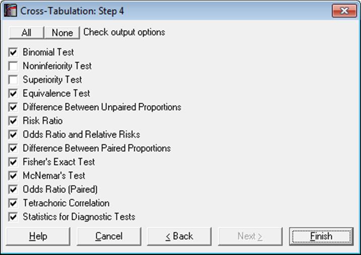
Example

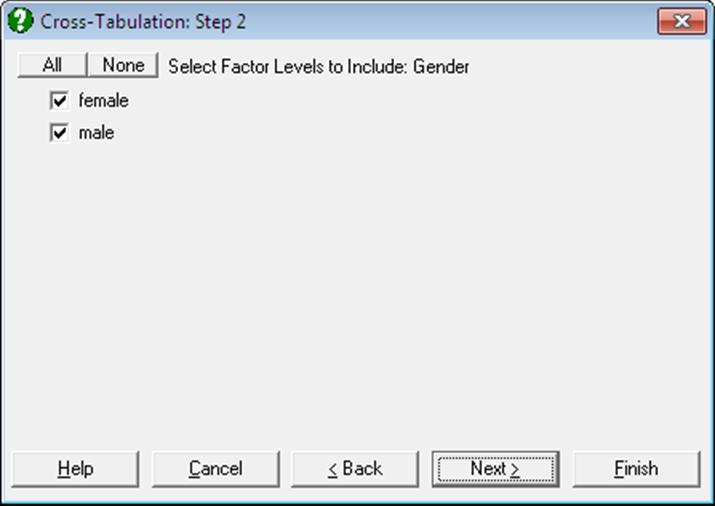
Open TABLES and select Statistics 1 → Tables → Cross-Tabulation. Select Gender (S12) as [Factor], Treatment (S13) as [Row Factor], Response (S14) as [Column Factor] and Count (C15) as [Weight]. At the next dialogue check all output options.

Output for the second stratum Gender = female is removed to save space.

Cross-Tabulation

Treatment (2 Rows) x Response (2 Columns)

Subsample selected by: Gender = female

 

Frequency

Treatment \ Response	Better	Same	Row Sum
Active	16.0000	11.0000	27.0000
Placebo	5.0000	20.0000	25.0000
Column Sum	21.0000	31.0000	52.0000

 

Expected

Treatment \ Response	Better	Same
Active	10.9038	16.0962
Placebo	10.0962	14.9038

 

Chi-Square

Treatment \ Response	Better	Same
Active	2.3818	1.6135
Placebo	2.5723	1.7426

 

Total %

Treatment \ Response	Better	Same	Row Sum
Active	30.77%	21.15%	51.92%
Placebo	9.62%	38.46%	48.08%
Column Sum	40.38%	59.62%	100.00%

 

Column %

Treatment \ Response	Better	Same
Active	76.19%	35.48%
Placebo	23.81%	64.52%

 

Row %

Treatment \ Response	Better	Same
Active	59.26%	40.74%
Placebo	20.00%	80.00%

 

Residuals

Treatment \ Response	Better	Same
Active	5.0962	-5.0962
Placebo	-5.0962	5.0962

 

Standardised Residuals

Treatment \ Response	Better	Same
Active	1.5433	-1.2702
Placebo	-1.6039	1.3201

 

Adjusted Residuals

Treatment \ Response	Better	Same
Active	2.8827	-2.8827
Placebo	-2.8827	2.8827

 

Chi-square Tests

	Chi-Square Statistic	Degrees of Freedom	Right-Tail Probability
Pearson	8.3102	1	0.0039
Likelihood-Ratio	8.6334	1	0.0033
Yates Correction	6.7595	1	0.0093
# Linear-by-linear	8.1504	1	0.0043
~ McNemar-Bowker

# Table scores

~ Reported for 3 x 3 or larger square tables.

Cells with expected count < 5 = 0 ( 0.00%)

Minimum expected count = 10.0962

 

Phi =	0.3998
Contingency Coefficient =	0.3712
Cramer's V =	0.3998

 

Fisher's Exact Test

	2-Tail Probability	Table Probability
Fisher's Exact	0.0052	0.0036

For an extended output see Fisher's exact test for 2 x 2 tables.

 

Measures of Association

	Value	Standard Error	Lower 95%	Upper 95%
Goodman-Kruskal's gamma	0.7067	0.1590	0.3951	1.0183
Kendall's tau b	0.3998	0.1247	0.1554	0.6441
Kendall's tau c	0.3920	0.1237	0.1495	0.6346
# Pearson Correlation	0.3998	0.1247	0.1554	0.6441
Spearman Rank Correlation	0.3998	0.1247	0.1554	0.6441
# Eta (col)	0.3998
# Eta (row)	0.3998
Somer's delta (col)	0.3926	0.1239	0.1498	0.6354
Somer's delta (row)	0.4071	0.1266	0.1590	0.6552
Somer's delta symmetric	0.3997	0.1246	0.1554	0.6440
Lambda (col)	0.2381	0.2160	-0.1852	0.6614
Lambda (row)	0.3600	0.1782	0.0108	0.7092
Lambda symmetric	0.3043	0.1729	-0.0346	0.6433
Uncertainty coefficient (col)	0.1231	0.0793	-0.0323	0.2784
Uncertainty coefficient (row)	0.1199	0.0775	-0.0320	0.2718
Uncertainty coefficient symmetric	0.1215	0.0783	-0.0321	0.2750

# Table scores

 

Cochran-Armitage Trend Test

	Z-Statistic	1-Tail Probability	2-Tail Probability
# Cochran-Armitage Trend Test	-1.2251	0.1103	0.2205

# Table scores

Binary variable is recoded to 0s and 1s.

Reported for 2 x K tables.

 

Cohen's Kappa

Expected Proportion =	0.4963
Observed Proportion =	0.6923

 

	Value	Standard Error	Z-Statistic	1-Tail Probability
Kappa	0.3891	0.1239	3.1404	0.0008

 

	2-Tail Probability	Lower 95%	Upper 95%
Kappa	0.0017	0.1463	0.6320

 

Binomial Test

For Treatment

Subsample selected by: Gender = female

 

Expected Proportion =	0.5000
Observed Proportion =	0.5192

 

	Proportion used in SE	Standard Error	Z-Statistic	1-Tail Probability
Wald	0.5192	0.0693
H0	0.5000	0.0693	0.2774	0.3908
Wald with CC	0.5192	0.0693
H0	0.5000	0.0693	0.1387	0.4449
Wilson (score)
Wilson with CC
Agresti-Coull	0.5179	0.0669
Agresti-Coull (+2)	0.5179	0.0668
Jeffreys
Clopper-Pearson (exact)				0.4449

 

	2-Tail Probability	Lower 95%	Upper 95%
Wald		0.3834	0.6550
H0	0.7815
Wald with CC		0.3738	0.6646
H0	0.8897
Wilson (score)		0.3869	0.6490
Wilson with CC		0.3778	0.6578
Agresti-Coull		0.3869	0.6490
Agresti-Coull (+2)		0.3870	0.6487
Jeffreys		0.3855	0.6509
Clopper-Pearson (exact)	0.8899	0.3763	0.6599

 

Binomial Test

For Response

Subsample selected by: Gender = female

 

Expected Proportion =	0.5000
Observed Proportion =	0.4038

 

	Proportion used in SE	Standard Error	Z-Statistic	1-Tail Probability
Wald	0.4038	0.0680
H0	0.5000	0.0693	-1.3868	0.0828
Wald with CC	0.4038	0.0680
H0	0.5000	0.0693	-1.2481	0.1060
Wilson (score)
Wilson with CC
Agresti-Coull	0.4105	0.0658
Agresti-Coull (+2)	0.4107	0.0657
Jeffreys
Clopper-Pearson (exact)				0.1058

 

	2-Tail Probability	Lower 95%	Upper 95%
Wald		0.2705	0.5372
H0	0.1655
Wald with CC		0.2609	0.5468
H0	0.2120
Wilson (score)		0.2816	0.5393
Wilson with CC		0.2731	0.5487
Agresti-Coull		0.2814	0.5395
Agresti-Coull (+2)		0.2819	0.5396
Jeffreys		0.2786	0.5394
Clopper-Pearson (exact)	0.2116	0.2701	0.5490

 

Difference Between Unpaired Proportions

Proportion 1 =	0.7619
Proportion 2 =	0.3548

 

	Difference	Standard Error	Z-Statistic	1-Tail Probability
Pooled Variance	0.4071	0.1412	2.8827	0.0020
Separate Variance		0.1266	3.2158	0.0007

 

	2-Tail Probability	Lower 95%	Upper 95%
Pooled Variance	0.0039	0.1303	0.6838
Separate Variance	0.0013	0.1590	0.6552

 

Risk Ratio

	Value	Lower 95%	Upper 95%
Risk Ratio	2.1472	1.2620	3.6533

 

Odds Ratio and Relative Risks

	Value	Lower 95%	Upper 95%
Odds Ratio	5.8182	1.6755	20.2034
Exact		1.4609	25.2654
Relative Risk (Cohort 1)	2.9630	1.2740	6.8913
Relative Risk (Cohort 2)	0.5093	0.3103	0.8357

 

Difference Between Paired Proportions

 

Proportion 1 =	0.2115
Proportion 2 =	0.0962

 

	Difference	Standard Error	Z-Statistic	1-Tail Probability
Normal Approximation	-0.1154	0.0752	-1.5000	0.0668
Exact Binomial				0.1051

 

	2-Tail Probability	Lower 95%	Upper 95%
Normal Approximation	0.1336	-0.2629	0.0321
Exact Binomial	0.2101	-0.2399	0.0533

 

Fisher's Exact Test

	Left-Tail	Right-Tail	Two-Tail	Table
Probability	0.9994	0.0042	0.0052	0.0036

 

McNemar's Test

	Chi-Square Statistic	Degrees of Freedom	Right-Tail Probability
Asymptotic	2.2500	1	0.1336
Asymptotic with CC	1.5625	1	0.2113

 

	2-Tail Probability	Lower 95%	Upper 95%
Exact Binomial	1.0000	0.7047	8.0769

 

Odds Ratio (Paired)

	Value	Lower 95%	Upper 95%
Odds Ratio (Paired)	0.4545	0.7047	8.0769

 

Tetrachoric Correlation

	Ratio	Tetrachoric Correlation
	5.8182	0.6052

 

Treatment (2 Rows) x Response (2 Columns)

Subsample selected by: Gender = male

 

. . .

Conditional Independence

	Chi-Square Statistic	Degrees of Freedom	Right-Tail Probability
Cochran	8.4650	1	0.0036
Mantel-Haenszel	7.1983	1	0.0073

 

Common Odds Ratio and Relative Risks

	Value	Standard Error	Lower 95%	Upper 95%
Common Odds Ratio	3.3132	0.4232	1.4456	7.5934
Cohort 1	2.1636	0.2867	1.2336	3.7948
Cohort 2	0.6420	0.1586	0.4705	0.8761
Logit(Odds Ratio)	3.2941	0.4300	1.4182	7.6515
Cohort 1	2.1059	0.2890	1.1951	3.7108
Cohort 2	0.6613	0.1580	0.4852	0.9013
Ln(Odds Ratio)	1.1979	0.4232	0.3685	2.0273

 

Homogeneity of Odds Ratio

	Chi-Square Statistic	Degrees of Freedom	Right-Tail Probability
Breslow-Day	1.4929	1	0.2218
Tarone	1.4905	1	0.2221