7.2.5. Logit / Probit / Gompit
Regressions with logit, probit, gompit (or complementary log log, cloglog) and loglog link functions can be estimated for models with binary dependent variables (dependent variables that consist of two values) as well as aggregated models where data contains a variable on the number of positive (or negative) responses and another variable giving the total number of subjects. All regressions work with similar inputs, employ the same maximum likelihood method and share the same output format, but differ in the link (objective) function used.
The logit and Logistic Regression procedures are closely related. A logit analysis with a binary dependent variable will produce the same coefficients estimated by Logistic Regression. For such problems use the Logistic Regression procedure if you need;
1) Receiver Operating Characteristic (ROC) and Sensitivity and Specificity curves, the area enclosed under the ROC curves (AUC), their confidence intervals and comparisons,
2) statistics for diagnostic tests,
3) odds ratios and their confidence intervals,
4) a classification table for the predicted and observed group memberships,
5) and a wide range of Case (Diagnostic) Statistics.
On the other hand, use the Logit / Probit / Gompit procedure if you need;
1) marginal and average effects,
2) to use data in aggregated (i.e. not in binary) format,
3) to estimate the heterogeneity factor (or dispersion parameter),
4) to estimate the natural response rate or
5) to estimate a probit, gompit (cloglog) or loglog model.
Like other regression options, Logit / Probit / Gompit also allows for automatic creation of interaction terms and dummy variables.
7.2.5.1. Logit / Probit / Gompit Model Description
The link functions described here are also available as axis scaling options in UNISTAT graphics engine (see Scale Type).
Logit: The logit function is an odds ratio for a given probability value:
Logit(p) = Ln(p/(1-p))
Logit(0.025) = -3.66
Logit(0.95) = 2.94.
Probit: This is the inverse standard cumulative normal distribution:
Probit(p) = Φ-1(p)
Probit(0.025) = -1.96
Probit(0.95) = 1.64
Gompit (Cloglog) : Unlike logit and probit, gompit is an asymmetric function:
Gompit(p) = Ln(-Ln(1-p))
Gompit(0.1) = -2.25
Gompit(0.9) = 0.834
Note that various sources interpret gompit, cloglog, loglog, nloglog in different ways. All these models are closely related to each other and one can obtain any of them by using the gompit link function.
For instance, if another source names complementary log log (cloglog) the function we call here gompit, one can switch between the two models by reversing the 0s and 1s in the dependent variable (in binary dependent variable models). This can be done without making any changes in data, by changing the encoding of the dependent variable on the Intermediate Inputs dialogue, by choosing the Max(Y) is encoded as 0 option.
Loglog:
Loglog(p) = -Ln(-Ln(p))
Loglog(0.1) = 2.25
Loglog(0.9) = -0.834
In models with binary dependent variable, one can switch between estimating a gompit model and a loglog model by reversing the 0s and 1s in the dependent variable and also reversing the signs of all independent variables (including the constant term).
A Newton-Raphson type maximum likelihood algorithm is employed to minimise the negative of the log likelihood function. The nature of this method implies that a solution (convergence) cannot always be achieved. In such cases, you are advised to edit the convergence parameters provided, in order to find the right levels for the particular problem at hand.
The logarithm of the likelihood function is:
![]()
and its first derivative:
![]()
where:
ri is the number of responses,
si is the number of subjects,
Fi is the inverse link function and
Gi is the first derivative of Fi.
Fi and Gi are defined for each link function as follows:
Logit:
![]()
![]()
Probit:
Normal cumulative probability function:
![]()
Normal density function:
![]()
Gompit (Cloglog):
![]()
![]()
Loglog:
![]()
![]()
With a binary dependent variable ri = yi (0 or 1) and si = 1.
7.2.5.2. Logit / Probit / Gompit Variable Selection
Logit / Probit / Gompit can analyse data in two different formats:
1) Binary (casewise) data where the dependent variable is a binary variable (it consists of two values), and
2) Aggregated (grouped) data, where similar cases are collapsed into groups to generate two columns, one containing the number of responses the other the total number of subjects in the group.
When the first data option is selected, the dependent variable should ideally contain only two distinct values (numeric or string). However, UNISTAT will accept any data column as the dependent variable and then, by default, encode internally those values which are equal to the minimum of this column as 0 and any other values as 1. Alternatively, you can make the program accept the maximum value as 1 and the rest as 0 by changing encoding of the dependent variable on the Intermediate Inputs dialogue by choosing the Max(Y) is encoded as 0 option.
This approach has the advantage and flexibility of running Logit / Probit / Gompit models on columns containing any type of categorical data. For instance, when a logit analysis is run on a column containing years 1995, 1996 and 1997, by default, UNISTAT will internally encode all 1995 entries as 0 and all 1996 and 1997 entries as 1. However, it is left to the user to ensure that the dependent variable selected contains sensible values.
The following is an example for the first data type, where there is one binary dependent variable and one independent variable:
|
Dependent |
Independent |
|
0 |
1.3 |
|
0 |
2.7 |
|
1 |
2.1 |
|
0 |
2.7 |
|
0 |
1.3 |
|
1 |
2.1 |
|
1 |
2.7 |
|
1 |
1.9 |
|
1 |
1.3 |
|
0 |
2.1 |
|
0 |
2.7 |
|
1 |
1.3 |
|
1 |
2.1 |
|
0 |
1.3 |
|
0 |
2.1 |
|
0 |
1.9 |
The same data set can be grouped (or collapsed) into the second (aggregated) format as follows:
|
Responses |
Subjects |
Independent |
|
2 |
5 |
1.3 |
|
1 |
2 |
1.9 |
|
3 |
5 |
2.1 |
|
1 |
4 |
2.7 |
where the first variable is called the response variable (which represents the number of true values within the group), and the second the subject variable (which represents the total number of cases in that group).
UNISTAT will first ask for the type of the dependent variable. If it is binary as described in (1) above, then select a dependent variable (by clicking on [Dependent]) which contains numeric or string categorical data, and any number of independent variables, which contain numeric data. If the data is in aggregated (or collapsed) from as described in (2) above, then select one column as Response (by clicking on [Response]) and one column as Subjects (by clicking on [Subject]). The following relation should hold for each case:
0 ≤ Response ≤ Subjects
Cases that do not conform to this (and Subjects = 0) will be considered as missing. As in Linear Regression, it is possible to create interaction terms and dummy variables, but not lag/lead terms (see 2.1.4. Creating Interaction, Dummy and Lag/Lead Variables).
It is also possible to select a factor (categorical) variable (by clicking on [Factor]) in which case the program will perform the analysis on a sub group as defined by the user (see 7.2.1.1. Linear Regression Variable Selection).
Next, an Intermediate Inputs dialogue will pop up. When the dependent variable is binary (and a dummy variable is selected), it will look as follows:
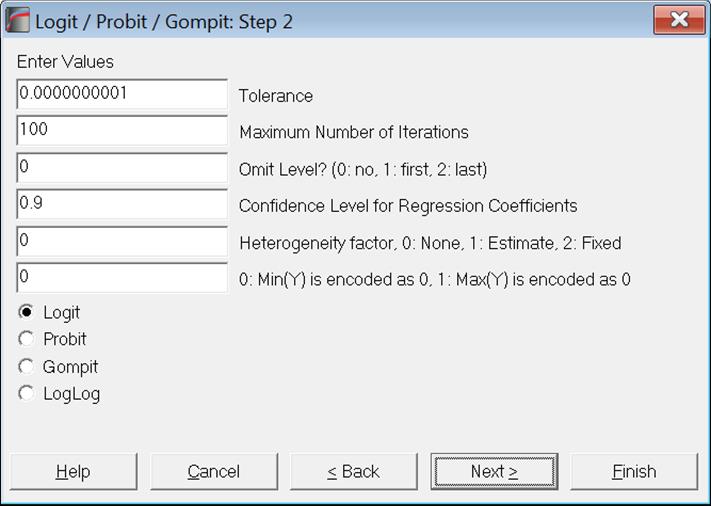
Tolerance: This value is used to control the sensitivity of nonlinear minimisation procedure employed. Under normal circumstances, you do not need to edit this value. If convergence cannot be achieved, then larger values of this parameter can be tried by removing one or more zeros.
Maximum Number of Iterations: When convergence cannot be achieved with the default value of 100 function evaluations, a higher value can be tried.
Omit Level: This box will appear only when one or more dummy variables have been included in the model from the Variable Selection Dialogue. Three options are available; (0) do not omit any levels, (1) omit the first level and (2) omit the last level. When no levels are omitted, the model will usually be over-parameterised (see 2.1.4. Creating Interaction, Dummy and Lag/Lead Variables).
Confidence Level for Regression Coefficients: While the general level of confidence (default 95%) is set on the Variable Selection Dialogue, confidence level for Regression Coefficients can be set here separately. The default is 90%.
Heterogeneity factor: This is also known as dispersion parameter. The default value of 0 means that a heterogeneity factor will not be used. If 1 is entered here, the heterogeneity factor will be estimated by the program. This is defined by default as:
Heterogeneity Factor = Deviance Chi-square / DoF.
However, sometimes this can also be defined as:
Heterogeneity Factor = Pearson Chi-square / DoF.
Although for a binary dependent variable these two values are the same, they differ for aggregated data option. If you want to estimate the heterogeneity factor by Pearson Chi-square, enter the following line in the [Options] section of Documents\Unistat10\Unistat10.ini file:
HeteroFactorPearson=1
Alternatively, you can also enter a given heterogeneity factor here (which is not 0 or 1) and the program will use the given value instead of estimating one.
If the heterogeneity factor is not zero, the covariance matrix will be multiplied by its square root. Therefore, regression coefficients will not be affected by this, but their standard errors will.
Dependent Variable Encoding: This box will appear only when the binary dependent variable option is selected. If this value is zero, the minimum of dependent variable is internally encoded as zero and any other value as 1. If the value in the box is nonzero, then the maximum of dependent variable is encoded as zero and any other value as 1.
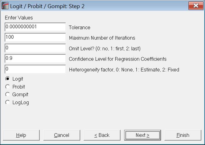
The Link Function: Select the model to be estimated. It can be one of logit, probit, gompit (cloglog) or loglog (see 7.2.5.1. Logit / Probit / Gompit Model Description).
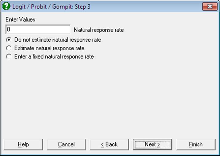
With the aggregated data option, a further dialogue is also displayed, asking whether a natural response rate is to be estimated or a fixed one will be given by the user. When a natural response rate is estimated, it will appear in the output just like any other estimated coefficient.
7.2.5.3. Logit / Probit / Gompit Output Options
For all models the following common regression output options are displayed.
Regression Coefficients:
The Z statistic is defined as:
![]()
If the heterogeneity factor is not zero, standard errors are multiplied by its square root. This is reported in the output.
The two-tailed normal probability value is:
![]()
The confidence intervals for regression coefficients are computed from:
![]()
where each coefficient’s standard error, ![]() , is the square root of the diagonal
element of the covariance matrix.
, is the square root of the diagonal
element of the covariance matrix.
Goodness of Fit Tests: See 7.2.6.4.1. Logistic Regression Results for details. Although for a binary dependent variable log-likelihood for initial and final model values are the same as Null Deviance and Deviance values respectively, they differ for aggregated data option.
Correlation Matrix for Regression Coefficients: Correlations between the estimated coefficients are displayed. If the heterogeneity factor is not zero, correlations are weighted by its square root.
Covariance Matrix for Regression Coefficients: Diagonal elements are the coefficient variances and off diagonal elements are the covariances between coefficients. If the heterogeneity factor is not zero, covariances are multiplied by it.
7.2.5.3.1. Output Options for Binary Dependent Variable
For a model with binary dependent variable, the following output options dialogue pops up.
Marginal Effects: This option is available for only binary dependent variable models. Marginal effects measure the change in the estimated probability when a change is made in independent variables. In other words, it is the partial derivative of the prediction function with respect to x:
![]()
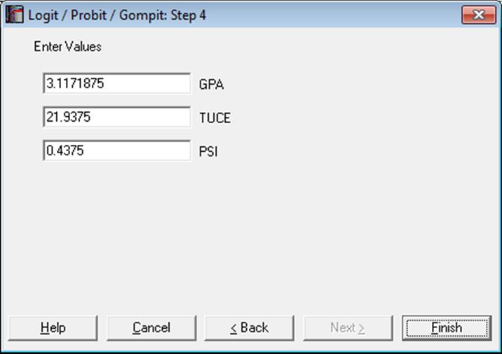
i.e., the estimated coefficient times its first derivative (slope) at x. You can enter values for the x-vector by clicking the [Opt] button situated to the left Marginal Effects output option. By default, the values displayed are the means of independent variables.
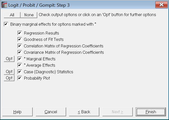
For dummy variables, or in general when an independent variable consists only of 0s and 1s, a slightly different procedure can be used, by checking the box Binary marginal effects for options marked with *. For details see p. 733, Greene (2012).
Average Effects: This option is available for only binary dependent variable models. Average effects are the sample mean of marginal effects computed for each case of the data.
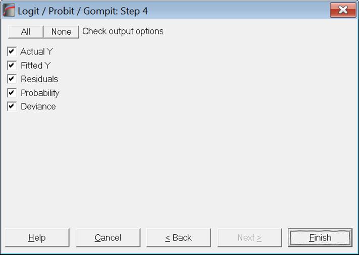
Case (Diagnostic) Statistics: Observed and expected responses, their differences and the expected probabilities are displayed. In models with a binary dependent variable, predictions are made for those cases where only the dependent variable is missing and no independent variables are missing. For further information see 7.2.6.4.2. Logistic Regression Case (Diagnostic) Statistics.
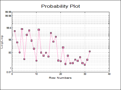
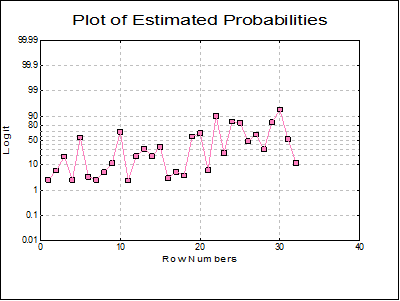
Plot of Estimated Probabilities: The estimated probabilities are plotted against the row numbers, using the appropriate link function for the scaling of the Left-Y axis.
7.2.5.3.2. Output Options for Aggregated Data
For models with aggregated data (i.e. the number of subjects and responses are given) the marginal and average effects options will not be available. When there are more than one independent variables, the Output Options Dialogue will look like this.
The case statistics table includes the subjects and responses data, as well as expected responses.
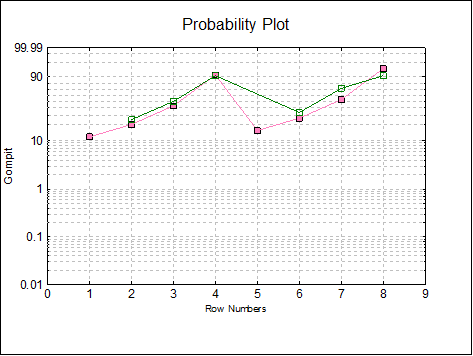
The Probability Plot displays observed and expected probabilities for each case in data. Probability values 0 and 1are considered missing.
7.2.5.4. Logit / Probit / Gompit Examples
Example 1
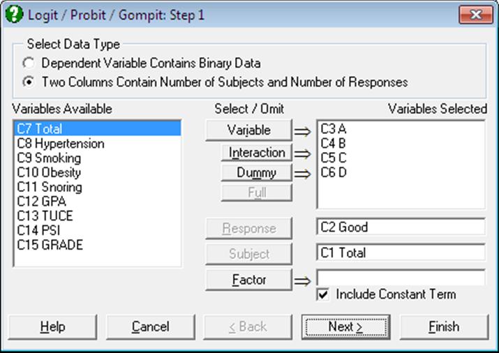
Table 12.19 on p. 353 from Altman & Douglas (1991). Open LOGIT, select Statistics 1 → Regression Analysis → Logit / Probit / Gompit and select the data option Two Columns Contain Number of Subjects and Number of Responses. Then select Total (C7) as [Subject], Hypertension (C8) as [Response] and Smoking, Obesity and Snoring (C9 to C11) as [Variable]s. Select Regression Results and Goodness of Fit Tests output options to obtain the following results:
Logit / Probit / Gompit
Model selected: Logit
Response Variable: Hypertension
Subject Variable: Total
Valid Number of Cases: 8, 0 Omitted
Regression Results
|
|
Coefficient |
Standard Error |
Z-Statistic |
2-Tail Probability |
Lower 90% |
Upper 90% |
|
Constant |
-2.3777 |
0.3802 |
-6.2540 |
0.0000 |
-3.0030 |
-1.7523 |
|
Smoking |
-0.0678 |
0.2781 |
-0.2437 |
0.8075 |
-0.5252 |
0.3897 |
|
Obesity |
0.6953 |
0.2851 |
2.4390 |
0.0147 |
0.2264 |
1.1642 |
|
Snoring |
0.8719 |
0.3976 |
2.1932 |
0.0283 |
0.2180 |
1.5259 |
Goodness of Fit Tests
|
|
-2 Log likelihood |
|
Initial Model |
411.4239 |
|
Final Model |
398.9164 |
|
|
Chi-Square Statistic |
Degrees of Freedom |
Right-Tail Probability |
|
Pearson |
1.3643 |
4 |
0.8504 |
|
Null Deviance |
14.1259 |
7 |
0.0490 |
|
Deviance |
1.6184 |
4 |
0.8055 |
|
Likelihood Ratio |
12.5075 |
3 |
0.0058 |
|
|
Pseudo R-squared |
|
McFadden |
0.0304 |
|
Adjusted McFadden |
0.0110 |
|
Cox & Snell |
0.0285 |
|
Nagelkerke |
0.0464 |
Go back to Variable Selection Dialogue, omit Smoking (C9) from the independent variable list and run the analysis again.
Logit / Probit / Gompit
Model selected: Logit
Response Variable: Hypertension
Subject Variable: Total
Valid Number of Cases: 8, 0 Omitted
Regression Results
|
|
Coefficient |
Standard Error |
Z-Statistic |
2-Tail Probability |
Lower 90% |
Upper 90% |
|
Constant |
-2.3921 |
0.3757 |
-6.3662 |
0.0000 |
-3.0101 |
-1.7740 |
|
Obesity |
0.6954 |
0.2851 |
2.4395 |
0.0147 |
0.2265 |
1.1643 |
|
Snoring |
0.8655 |
0.3967 |
2.1819 |
0.0291 |
0.2130 |
1.5179 |
Goodness of Fit Tests
|
|
-2 Log likelihood |
|
Initial Model |
411.4239 |
|
Final Model |
398.9761 |
|
|
Chi-Square Statistic |
Degrees of Freedom |
Right-Tail Probability |
|
Pearson |
1.3854 |
5 |
0.9259 |
|
Null Deviance |
14.1259 |
7 |
0.0490 |
|
Deviance |
1.6781 |
5 |
0.8916 |
|
Likelihood Ratio |
12.4478 |
2 |
0.0020 |
|
|
Pseudo R-squared |
|
McFadden |
0.0303 |
|
Adjusted McFadden |
0.0157 |
|
Cox & Snell |
0.0283 |
|
Nagelkerke |
0.0462 |
Example 2
Example 14.1 on p. 490 from Armitage & Berry (2002). Data given in Table 14.1 needs to be transformed into a suitable format where the main effects of the four factors A, B, C and D can be analysed. This is done by creating a new column for each factor such that it contains the value one if the factor occurs in the factor combination column and zero otherwise. The data matrix would then look like this:
|
Total |
Good |
A |
B |
C |
D |
|
477 |
84 |
0 |
0 |
0 |
0 |
|
231 |
75 |
1 |
0 |
0 |
0 |
|
63 |
13 |
0 |
1 |
0 |
0 |
|
94 |
35 |
1 |
1 |
0 |
0 |
|
150 |
67 |
0 |
0 |
1 |
0 |
|
378 |
201 |
1 |
0 |
1 |
0 |
|
32 |
16 |
0 |
1 |
1 |
0 |
|
169 |
102 |
1 |
1 |
1 |
0 |
|
12 |
2 |
0 |
0 |
0 |
1 |
|
13 |
7 |
1 |
0 |
0 |
1 |
|
7 |
4 |
0 |
1 |
0 |
1 |
|
12 |
8 |
1 |
1 |
0 |
1 |
|
11 |
3 |
0 |
0 |
1 |
1 |
|
45 |
27 |
1 |
0 |
1 |
1 |
|
4 |
1 |
0 |
1 |
1 |
1 |
|
31 |
23 |
1 |
1 |
1 |
1 |
Open LOGIT, select Statistics 1 → Regression Analysis → Logit / Probit / Gompit and select the data option Two Columns Contain Number of Subjects and Number of Responses. Then select Total (C1) as [Subject], Good (C2) as [Response] and A, B, C, D (C3 to C6) as [Variable]s. Select all output options for the following results:
Logit / Probit / Gompit
Model selected: Logit
Response Variable: Good
Subject Variable: Total
Valid Number of Cases: 16, 0 Omitted
Regression Results
|
|
Coefficient |
Standard Error |
Z-Statistic |
2-Tail Probability |
Lower 90% |
Upper 90% |
|
Constant |
-1.4604 |
0.0964 |
-15.1490 |
0.0000 |
-1.6190 |
-1.3019 |
|
A |
0.6498 |
0.1154 |
5.6298 |
0.0000 |
0.4599 |
0.8396 |
|
B |
0.3101 |
0.1222 |
2.5377 |
0.0112 |
0.1091 |
0.5111 |
|
C |
0.9806 |
0.1107 |
8.8560 |
0.0000 |
0.7985 |
1.1627 |
|
D |
0.4204 |
0.1910 |
2.2011 |
0.0277 |
0.1062 |
0.7345 |
Goodness of Fit Tests
|
|
-2 Log likelihood |
|
Initial Model |
2306.7889 |
|
Final Model |
2104.1204 |
|
|
Chi-Square Statistic |
Degrees of Freedom |
Right-Tail Probability |
|
Pearson |
13.6067 |
11 |
0.2555 |
|
Null Deviance |
216.2594 |
15 |
0.0000 |
|
Deviance |
13.5909 |
11 |
0.2565 |
|
Likelihood Ratio |
202.6685 |
4 |
0.0000 |
|
|
Pseudo R-squared |
|
McFadden |
0.0879 |
|
Adjusted McFadden |
0.0835 |
|
Cox & Snell |
0.1106 |
|
Nagelkerke |
0.1106 |
Correlation Matrix of Regression Coefficients
|
|
Constant |
A |
B |
C |
D |
|
Constant |
1.0000 |
-0.5095 |
-0.1961 |
-0.3929 |
-0.0716 |
|
A |
-0.5095 |
1.0000 |
-0.1534 |
-0.2952 |
-0.0430 |
|
B |
-0.1961 |
-0.1534 |
1.0000 |
-0.0014 |
-0.0810 |
|
C |
-0.3929 |
-0.2952 |
-0.0014 |
1.0000 |
-0.0569 |
|
D |
-0.0716 |
-0.0430 |
-0.0810 |
-0.0569 |
1.0000 |
Covariance Matrix of Regression Coefficients
|
|
Constant |
A |
B |
C |
D |
|
Constant |
0.0093 |
-0.0057 |
-0.0023 |
-0.0042 |
-0.0013 |
|
A |
-0.0057 |
0.0133 |
-0.0022 |
-0.0038 |
-0.0009 |
|
B |
-0.0023 |
-0.0022 |
0.0149 |
-0.0000 |
-0.0019 |
|
C |
-0.0042 |
-0.0038 |
-0.0000 |
0.0123 |
-0.0012 |
|
D |
-0.0013 |
-0.0009 |
-0.0019 |
-0.0012 |
0.0365 |
Case (Diagnostic) Statistics
|
|
Subjects |
Responses |
Expected Responses |
Residuals |
Probability |
Deviance |
|
1 |
477 |
84 |
89.8673 |
-5.8673 |
0.1884 |
-0.6929 |
|
2 |
231 |
75 |
71.0915 |
3.9085 |
0.3078 |
0.5544 |
|
3 |
63 |
13 |
15.1470 |
-2.1470 |
0.2404 |
-0.6440 |
|
4 |
94 |
35 |
35.4771 |
-0.4771 |
0.3774 |
-0.1016 |
|
5 |
150 |
67 |
57.3442 |
9.6558 |
0.3823 |
1.6077 |
|
6 |
378 |
201 |
205.0245 |
-4.0245 |
0.5424 |
-0.4153 |
|
7 |
32 |
16 |
14.6455 |
1.3545 |
0.4577 |
0.4797 |
|
8 |
169 |
102 |
104.4028 |
-2.4028 |
0.6178 |
-0.3795 |
|
9 |
12 |
2 |
3.1336 |
-1.1336 |
0.2611 |
-0.7812 |
|
10 |
13 |
7 |
5.2474 |
1.7526 |
0.4036 |
0.9794 |
|
11 |
7 |
4 |
2.2764 |
1.7236 |
0.3252 |
1.3364 |
|
12 |
12 |
8 |
5.7596 |
2.2404 |
0.4800 |
1.3035 |
|
13 |
11 |
3 |
5.3365 |
-2.3365 |
0.4851 |
-1.4390 |
|
14 |
45 |
27 |
28.9549 |
-1.9549 |
0.6434 |
-0.6034 |
|
15 |
4 |
1 |
2.2493 |
-1.2493 |
0.5623 |
-1.2690 |
|
16 |
31 |
23 |
22.0422 |
0.9578 |
0.7110 |
0.3838 |
Next go back to the Variable Selection Dialogue and check the Probit option. Select only the Regression Results output option.
Logit / Probit / Gompit
Model selected: Probit
Response Variable: Good
Subject Variable: Total
Valid Number of Cases: 16, 0 Omitted
Regression Results
|
|
Coefficient |
Standard Error |
Z-Statistic |
2-Tail Probability |
Lower 90% |
Upper 90% |
|
Constant |
-0.8933 |
0.0561 |
-15.9286 |
0.0000 |
-0.9855 |
-0.8010 |
|
A |
0.3963 |
0.0698 |
5.6740 |
0.0000 |
0.2814 |
0.5112 |
|
B |
0.1890 |
0.0749 |
2.5238 |
0.0116 |
0.0658 |
0.3123 |
|
C |
0.6027 |
0.0675 |
8.9292 |
0.0000 |
0.4917 |
0.7137 |
|
D |
0.2584 |
0.1169 |
2.2106 |
0.0271 |
0.0661 |
0.4508 |
Example 3
Example 17.3 on p. 735 Greene (2012). Tables 17.1 and 17.2 display results for three link functions. As these tables contain some misprints, the user is advised to validate the results with the book’s errata website.
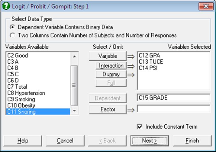
Open LOGIT, select Statistics 1 → Regression Analysis → Logit / Probit / Gompit and select the data option Dependent Variable Contains Binary Data. Then select GRADE (C15) as [Dependent] and GPA, TUCE and PSI (C12 to C14) as [Variable]s. Select Logit and all output options.
Logit / Probit / Gompit
Model selected: Logit
Dependent Variable: GRADE
Minimum of dependent variable is encoded as 0 and the rest as 1.
Valid Number of Cases: 32, 0 Omitted
Regression Results
|
|
Coefficient |
Standard Error |
Z-Statistic |
2-Tail Probability |
Lower 90% |
Upper 90% |
|
Constant |
-13.0213 |
4.9313 |
-2.6405 |
0.0083 |
-21.1327 |
-4.9100 |
|
GPA |
2.8261 |
1.2629 |
2.2377 |
0.0252 |
0.7488 |
4.9035 |
|
TUCE |
0.0952 |
0.1416 |
0.6722 |
0.5014 |
-0.1377 |
0.3280 |
|
PSI |
2.3787 |
1.0646 |
2.2344 |
0.0255 |
0.6276 |
4.1297 |
Goodness of Fit Tests
|
|
-2 Log likelihood |
|
Initial Model |
41.1835 |
|
Final Model |
25.7793 |
|
|
Chi-Square Statistic |
Degrees of Freedom |
Right-Tail Probability |
|
Pearson |
27.2571 |
28 |
0.5043 |
|
Null Deviance |
41.1835 |
31 |
0.1045 |
|
Deviance |
25.7793 |
28 |
0.5852 |
|
Likelihood Ratio |
15.4042 |
3 |
0.0015 |
|
|
Pseudo R-squared |
|
McFadden |
0.3740 |
|
Adjusted McFadden |
0.1798 |
|
Cox & Snell |
0.3821 |
|
Nagelkerke |
0.5278 |
Correlation Matrix of Regression Coefficients
|
|
Constant |
GPA |
TUCE |
PSI |
|
Constant |
1.0000 |
-0.7343 |
-0.4960 |
-0.4494 |
|
GPA |
-0.7343 |
1.0000 |
-0.2065 |
0.3181 |
|
TUCE |
-0.4960 |
-0.2065 |
1.0000 |
0.0990 |
|
PSI |
-0.4494 |
0.3181 |
0.0990 |
1.0000 |
Covariance Matrix of Regression Coefficients
|
|
Constant |
GPA |
TUCE |
PSI |
|
Constant |
24.3180 |
-4.5735 |
-0.3463 |
-2.3592 |
|
GPA |
-4.5735 |
1.5950 |
-0.0369 |
0.4276 |
|
TUCE |
-0.3463 |
-0.0369 |
0.0200 |
0.0149 |
|
PSI |
-2.3592 |
0.4276 |
0.0149 |
1.1333 |
Marginal Effects
|
|
Coefficient |
Standard Error |
Z-Statistic |
2-Tail Probability |
Lower 90% |
Upper 90% |
X |
|
GPA |
0.5339 |
0.2370 |
2.2522 |
0.0243 |
0.1440 |
0.9238 |
3.1172 |
|
TUCE |
0.0180 |
0.0262 |
0.6851 |
0.4933 |
-0.0252 |
0.0611 |
21.9375 |
|
* PSI |
0.4565 |
0.1811 |
2.5213 |
0.0117 |
0.1587 |
0.7543 |
0.4375 |
|
x’B = |
-1.0836 |
|
Predicted Probability = |
0.2528 |
|
f*x’B = |
-0.2047 |
|
Predicted Marginal Probability = |
0.4490 |
* Binary Independent Variable
Average Effects
|
|
Coefficient |
Standard Error |
Z-Statistic |
2-Tail Probability |
Lower 90% |
Upper 90% |
|
GPA |
0.3626 |
0.1094 |
3.3130 |
0.0009 |
0.1826 |
0.5426 |
|
TUCE |
0.0122 |
0.0178 |
0.6861 |
0.4927 |
-0.0171 |
0.0415 |
|
* PSI |
0.3575 |
0.1420 |
2.5177 |
0.0118 |
0.1239 |
0.5911 |
* Binary Independent Variable
Case (Diagnostic) Statistics
|
|
Actual Y |
Fitted Y |
Residuals |
Probability |
Deviance |
|
1 |
0 |
0.0266 |
-0.0266 |
0.0266 |
-0.2321 |
|
2 |
0 |
0.0595 |
-0.0595 |
0.0595 |
-0.3503 |
|
3 |
0 |
0.1873 |
-0.1873 |
0.1873 |
-0.6440 |
|
… |
… |
… |
… |
… |
… |
|
30 |
1 |
0.9453 |
0.0547 |
0.9453 |
0.3353 |
|
31 |
0 |
0.5291 |
-0.5291 |
0.5291 |
-1.2273 |
|
32 |
1 |
0.1110 |
0.8890 |
0.1110 |
2.0966 |
Now select Probit and Gompit link functions with only the Regression Results, Marginal Effects output options.
Logit / Probit / Gompit
Model selected: Probit
Dependent Variable: GRADE
Minimum of dependent variable is encoded as 0 and the rest as 1.
Valid Number of Cases: 32, 0 Omitted
Regression Results
|
|
Coefficient |
Standard Error |
Z-Statistic |
2-Tail Probability |
Lower 90% |
Upper 90% |
|
Constant |
-7.4523 |
2.5425 |
-2.9311 |
0.0034 |
-11.6343 |
-3.2703 |
|
GPA |
1.6258 |
0.6939 |
2.3431 |
0.0191 |
0.4845 |
2.7671 |
|
TUCE |
0.0517 |
0.0839 |
0.6166 |
0.5375 |
-0.0863 |
0.1897 |
|
PSI |
1.4263 |
0.5950 |
2.3970 |
0.0165 |
0.4476 |
2.4051 |
Marginal Effects
|
|
Coefficient |
Standard Error |
Z-Statistic |
2-Tail Probability |
Lower 90% |
Upper 90% |
X |
|
GPA |
0.5333 |
0.2325 |
2.2943 |
0.0218 |
0.1510 |
0.9157 |
3.1172 |
|
TUCE |
0.0170 |
0.0271 |
0.6257 |
0.5315 |
-0.0276 |
0.0616 |
21.9375 |
|
* PSI |
0.4644 |
0.1703 |
2.7274 |
0.0064 |
0.1843 |
0.7445 |
0.4375 |
|
x’B = |
-0.6255 |
|
Predicted Probability = |
0.2658 |
|
f*x’B = |
-0.2052 |
|
Predicted Marginal Probability = |
0.4187 |
* Binary Independent Variable
Logit / Probit / Gompit
Model selected: Gompit
Dependent Variable: GRADE
Minimum of dependent variable is encoded as 0 and the rest as 1.
Valid Number of Cases: 32, 0 Omitted
Regression Results
|
|
Coefficient |
Standard Error |
Z-Statistic |
2-Tail Probability |
Lower 90% |
Upper 90% |
|
Constant |
-10.0314 |
3.4791 |
-2.8834 |
0.0039 |
-15.7540 |
-4.3089 |
|
GPA |
2.2936 |
1.0350 |
2.2160 |
0.0267 |
0.5911 |
3.9960 |
|
TUCE |
0.0412 |
0.1073 |
0.3835 |
0.7013 |
-0.1354 |
0.2177 |
|
PSI |
1.5623 |
0.7305 |
2.1386 |
0.0325 |
0.3607 |
2.7639 |
Marginal Effects
|
|
Coefficient |
Standard Error |
Z-Statistic |
2-Tail Probability |
Lower 90% |
Upper 90% |
X |
|
GPA |
0.4775 |
0.2031 |
2.3509 |
0.0187 |
0.1434 |
0.8115 |
3.1172 |
|
TUCE |
0.0086 |
0.0222 |
0.3865 |
0.6991 |
-0.0279 |
0.0450 |
21.9375 |
|
* PSI |
0.3536 |
0.1610 |
2.1958 |
0.0281 |
0.0887 |
0.6185 |
0.4375 |
|
x’B = |
-1.2956 |
|
Predicted Probability = |
0.2395 |
|
f*x’B = |
-0.2697 |
|
Predicted Marginal Probability = |
0.5340 |
* Binary Independent Variable
Now select Probit and Gompit link functions, uncheck the Binary marginal effects box and only the Marginal Effects output option.
Logit / Probit / Gompit
Model selected: Logit
Dependent Variable: GRADE
Minimum of dependent variable is encoded as 0 and the rest as 1.
Valid Number of Cases: 32, 0 Omitted
Marginal Effects
|
|
Coefficient |
Standard Error |
Z-Statistic |
2-Tail Prob |
Lower 90% |
Upper 90% |
X |
|
GPA |
0.5339 |
0.2370 |
2.2522 |
0.0243 |
0.1440 |
0.9238 |
3.1172 |
|
TUCE |
0.0180 |
0.0262 |
0.6851 |
0.4933 |
-0.0252 |
0.0611 |
21.9375 |
|
PSI |
0.4493 |
0.1968 |
2.2837 |
0.0224 |
0.1587 |
0.7543 |
0.4375 |
|
x’B = |
-1.0836 |
|
Predicted Probability = |
0.2528 |
|
f*x’B = |
-0.2047 |
|
Predicted Marginal Probability = |
0.4490 |
Logit / Probit / Gompit
Model selected: Probit
Dependent Variable: GRADE
Minimum of dependent variable is encoded as 0 and the rest as 1.
Valid Number of Cases: 32, 0 Omitted
Marginal Effects
|
|
Coefficient |
Standard Error |
Z-Statistic |
2-Tail Prob |
Lower 95% |
Upper 95% |
X |
|
GPA |
0.5333 |
0.2325 |
2.2943 |
0.0218 |
0.1510 |
0.9157 |
3.1172 |
|
TUCE |
0.0170 |
0.0271 |
0.6257 |
0.5315 |
-0.0276 |
0.0616 |
21.9375 |
|
PSI |
0.4679 |
0.1876 |
2.4936 |
0.0126 |
0.1843 |
0.7445 |
0.4375 |
|
x’B = |
-0.6255 |
|
Predicted Probability = |
0.2658 |
|
f*x’B = |
-0.2052 |
|
Predicted Marginal Probability = |
0.4187 |