7.2.1. Linear Regression
The Linear Regression procedure is suitable for estimating weighted or nonweighted linear regression models with or without a constant term, including nonlinear models such as multiplicative, exponential or reciprocal regressions that can be linearised by logarithmic or exponential transformations. It is possible to run regressions without an independent variable, which is equivalent to running a noconstant regression against a unity independent variable.
Regressions may be run on a subset of cases as determined by the combination of levels of an unlimited number of factor columns. An unlimited number of dependent variables can be selected to run the same model on different dependent variables. It is also possible to include interaction terms, dummy and lag/lead variables in the model, without having to create them as data columns in the spreadsheet first.
The output includes a wide range of graphics and statistics options. In regression plots, it is possible to omit outliers interactively, by pressing down the right mouse button on a data point and then pressing <Delete>.
7.2.1.1. Linear Regression Variable Selection
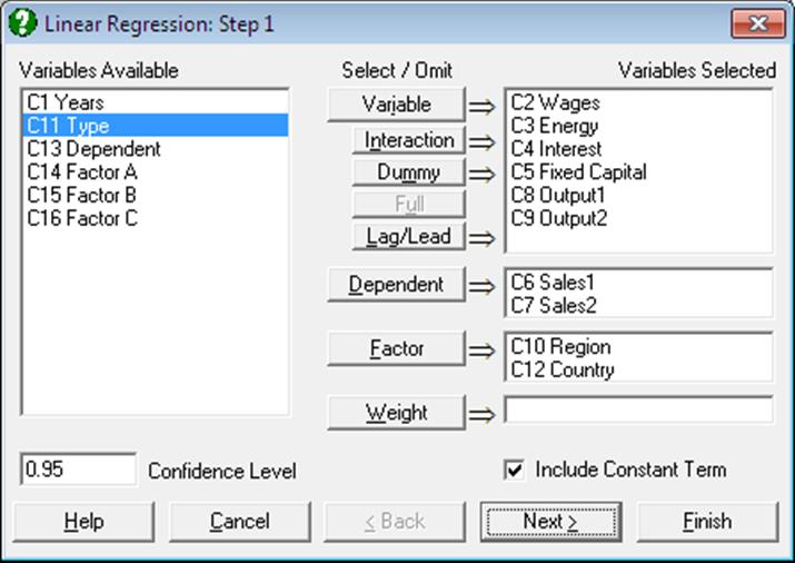
All columns selected for this procedure should have an equal size. The buttons on the Variable Selection Dialogue have the following tasks:
Variable: Click on [Variable] to select a column containing continuous numeric data as an independent variable.
Interaction: This button is used to create independent variables, which are the products of existing numeric variables. If only one variable is highlighted, then the new independent variable created will be the product of the selected variable by itself. If two or more variables are highlighted, then the new term will be the product of these variables. Maximum three-way interactions are allowed. Interactions of dummy variables or lags are not allowed. In order to create interaction terms for dummy variables, create interactions first, and then create dummy variables for them. For further information see 2.1.4. Creating Interaction, Dummy and Lag/Lead Variables.
Dummy: This button is used to create n or n – 1 new independent (dummy or indicator) variables for a factor column containing n levels. Each dummy variable corresponds to a level of the factor column. A case in a dummy column will have the value of 1 if the factor contains the corresponding level in the same row, and 0 otherwise. If the selected variable is an interaction term, then dummy variables will be created for this interaction term. Up to three-way interactions are allowed and columns containing short or Long Strings can be selected as factors. It is possible to include all n levels or to omit the first or the last level in order to remove the inherent over-parameterisation of the model. For further information see 2.1.4. Creating Interaction, Dummy and Lag/Lead Variables.
Full: This button becomes activated when two or more categorical variables are highlighted. Like the [Dummy] button, it is also used to create dummy variables. The only difference is that this button will create all necessary dummy variables and their interactions to specify a complete model. For instance, if two categorical variables are highlighted, this button will create two sets of dummy variables representing the main effects and a third set representing the interaction term between the two factors. Maximum three-way interactions are supported.
Lag/Lead: This button is used to create new independent variables by shifting the rows of an existing variable up or down. When a lag variable is specified in the Variable Selection Dialogue, then a further dialogue will ask for the number of lags (or leads) for each item selected. Negative integers represent the lags and positive integers the leads. For further information see 2.1.4. Creating Interaction, Dummy and Lag/Lead Variables.
Dependent: It is compulsory to select at least one column containing numeric data as a dependent variable. When more than one dependent variable is selected, the analysis will be repeated as many times as the number of dependent variables, each time only changing the dependent variable and keeping the rest of selections unchanged.
Factor: This allows you to run regressions on subsamples of rows (cases). With some time series or panel data it is desirable to run regressions on some, rather than all rows of the data matrix. Although it is possible to extract subsets using a Data Processor function such as If() (see 3.4.2.7. Conditional Functions), Data → Recode Column, Subsample Save (see 2.4.1.6.3. Options) or Data → Select Row, it is much more convenient to use the selection facility provided here.
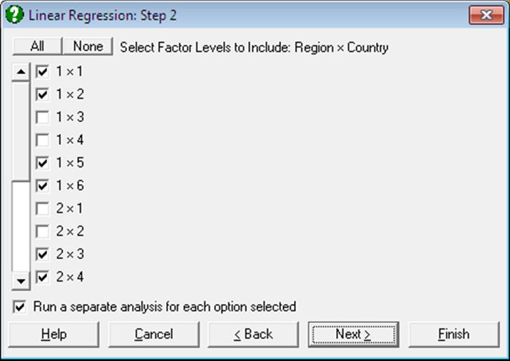
To make use of this facility the data matrix should contain at least one factor column. An unlimited number of factors can be selected. These can be numeric or String Data columns, but each column must contain a limited number of distinct values. Select the factor columns from the Variables Available list by clicking on [Factor]. Then the program will display a dialogue where all possible combinations of factor levels are displayed in a list of check boxes. For instance, if one factor containing three levels is selected, only three check boxes will be displayed representing each level. Only the rows of data matrix corresponding to the checked levels will be included in the regression. If there are two factors selected, say one having two levels and the other three, then the list will contain six check boxes, 1×1, 1×2, 1×3, 2×1, 2×2, 2×3. Suppose the check boxes 1×2 and 2×2 are checked. Then only those rows of the data matrix containing 1 in the first factor column and 2 in the second and 2 in the first factor and 2 in the second will be included in the regression. When more than one selection is made, it is possible to run a single Regression Analysis on all selected rows combined, or to run a separate analysis for each selection.
With subsample selection, the possibility of getting an Insufficient degrees of freedom message will increase considerably. Also, interpretation of the Durbin-Watson statistic may not be obvious.
Weight: It was mentioned at the beginning of this chapter that when a column is selected as a weights variable, the program will normalise this column so that its sum is equal to the number of valid cases, and then multiply each independent variable by its square root. In a weighted regression run with constant term included, the column of 1s in the X matrix should also be multiplied by the square root of weights, as the Regression Analysis considers the constant term just like any other coefficient. The algorithm used here produces exactly the same effect without having to take the square root of weights, thus achieving higher accuracy.
7.2.1.2. Linear Regression Output Options
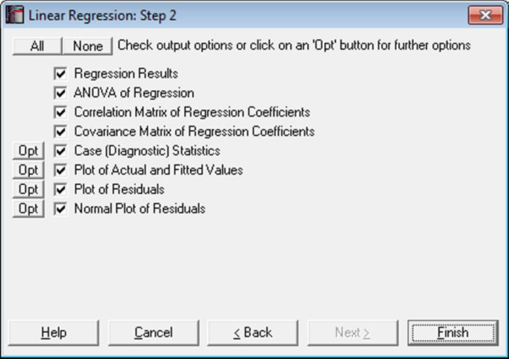
An Output Options Dialogue will provide access to the following options. The Actual and Fitted Values, Residuals and Confidence Intervals for Mean and Actual Y Values options that existed in earlier versions of UNISTAT have now been merged under the Case (Diagnostic) Statistics option. See 7.2.1.2.2. Linear Regression Case Output.
Multicollinearity: One of the basic assumptions of the method of least squares estimation is that no linear dependency exists between the regression variables. However, the present implementation will detect the variables causing multicollinearity and display them at the end of coefficients table. If you do not wish to display these variables enter the following line in the [Options] section of Documents\Unistat10\Unistat10.ini file:
DispCollin=0
The rest of the coefficients will be determined as if the regression were run without the variables causing collinearity.
Perfect Fit: If the current set of independent variables fully explain the variation of the dependent variable, the program displays a restricted number of results options, main results themselves being confined to estimated regression coefficients only.
Perfect fit will be reported under the following two circumstances;
1) if R-squared > 0.99999 or
2) if the number of variables (including the dependent variable) is equal to the number of observations, in which case R-squared is not computed.
7.2.1.2.1. Linear Regression Coefficient Output
Regression Results: The main regression output displays a table for coefficients of the estimated regression equation, their standard errors, t-statistics, probability values (from the t-distribution) and confidence intervals for the significance level specified in the regression Variable Selection Dialogue. If any independent variables have been omitted due to multicollinearity, they are reported at the end of the table. If you do not wish to display these variables enter the following line in the [Options] section of Documents\Unistat10\Unistat10.ini file:
DispCollin=0
When the model contains dummy variables with very long string values, output may look cramped. You can display the numbers of levels, instead of their string values, by entering the following line in the [Options] section of Unistat10.ini:
OLSFullLabel=0
In Stand-Alone Mode, the estimated regression coefficients can be saved to data matrix by clicking on the UNISTAT icon (which becomes visible on the right of the toolbar in Output Window and Data Processor after running a procedure). The same coefficients will also be saved automatically in the file POLYCOEF.TXT, in the order of C0 (constant term, if any), C1, C2, …, Cr.
The rest of the output consists of the following statistics: residual sum of squares, standard error of regression, mean and standard deviation of the dependent variable, R-squared, R-squared adjusted for the degrees of freedom, F-statistic and its tail probability, the Durbin-Watson statistic, press statistic and the log of likelihood function. The Durbin-Watson statistic will be adjusted for the number of gaps in data caused by missing values. The number of rows omitted due to missing values is reported if it is other than zero.
ANOVA of Regression: The total variation of the dependent variable is partitioned into the Regression (or explained) part which is due to the linear influence of independent variables and the Error (or unexplained) part which is expressed in residuals.
The F-value is the ratio of the mean squares for regression and mean squares for the error term. The null hypothesis of “no relationship between the dependent variable and independent variables as a whole” can be tested by means of the probability value reported.
Individual contributions of independent variables to the regression (explained) sum of squares are also displayed. The sum of individual contributions will be equal to the regression sum of squares. However, it is important here to emphasise that these individual contributions are specific to the order in which independent variables enter into the regression equation. Normally, when two independent variables change place, their individual contributions to the regression sum of squares will also change.
Correlation Matrix of Regression Coefficients: This is a symmetric matrix with unity diagonal elements. It gives the correlation between the regression coefficients and is obtained by dividing the elements of (X’X)-1 matrix by the square root of the diagonal elements corresponding to its row and column.
Covariance Matrix of Regression Coefficients: This option displays a symmetric matrix where diagonal elements are the variances and off-diagonal elements are the covariances of the estimated regression coefficients. This matrix is sometimes referred to as the dispersion matrix and it can also be obtained by multiplying (X’X)-1 matrix by the estimated variance of the error terms.
7.2.1.2.2. Linear Regression Case Output
Case (Diagnostic) Statistics: These statistics are useful in determining the influence of individual observations on the overall fit of the model. Looking at outliers (cases with a large residual value) is an effective way of determining whether the model fitted explains well the variation in data. However, residuals alone cannot explain all types of influence of individual cases on the regression. Suppose, for instance, a data set where most observations are clustered together but only one point lies outside the cluster. Suppose also that the regression line passes near this point so that it does not have a large residual. Nevertheless, removing this single point from the regression may have substantial effects on the estimated coefficients (called leverage).
Most of the regression diagnostic statistics below measure such effects, which answer the question what would happen if this case was removed from the regression. Luckily, we do not need to estimate the entire model after deleting each case, but compute the same results by applying the following algebraic manipulations.
Let:
n = valid number of cases and
m = number of coefficients in the model.
Therefore:
m = 1 + number of independent variables (with constant) and
m = number of independent variables (with no constant).
Also, each row of the data matrix is defined as:
Xi = 1+X1i,…,Xm-1i for regressions with constant and
Xi = X1i,…,Xmi for regressions without constant.
Central to most diagnostic statistics are definitions of root mean square of residuals:
![]()
and the diagonal vector of the projection matrix:
![]()
Predictions (Interpolations): There are three conditions under which predictions will be computed for estimated Y values:
1) If, for a case, all independent variables are non-missing, but only the dependent variable is missing,
2) If a case does not contain missing values but it has been omitted from the analysis by Data Processor’s Data → Select Row function,
3) If a case does not contain missing values but it has been omitted from the analysis by selecting subsamples from the Variable Selection Dialogue (see 2.1.2. Categorical Data Analysis).
Such cases are not included in the estimation of the model. When, however, Case (Diagnostic) Statistics option is selected, the program will detect these cases and compute and display the fitted (estimated) Y values, as well as their confidence intervals and some other related statistics. Therefore, it will be a good idea to include the cases for which predictions are to be made in the data matrix during the data preparation phase, and then exclude them from the analysis by one of the above three methods. When a case is predicted, its label will be prefixed by an asterisk (*).
In Stand-Alone Mode, the spreadsheet function Reg can also be used to make predictions (see 3.4.2.6.3. UNISTAT Functions).
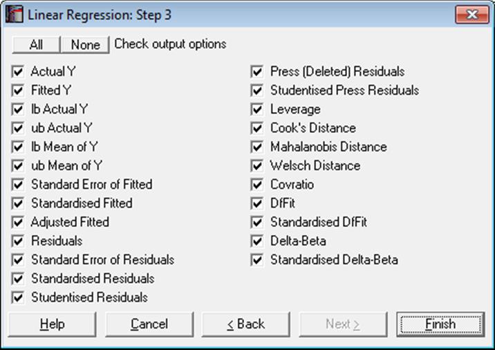
Statistics available under Case (Diagnostic) Statistics option are as follows.
Actual Y: Observed values of the dependent variable.
![]()
Fitted Y: Estimated values of the dependent variable.
![]()
Confidence Intervals for Actual Y-values:
![]()
where X is the given vector of independent variable
values, β is the vector of estimated coefficients, ![]() is
the critical value from the t-distribution for an α / 2 level of
significance and n – k degrees of freedom and S is the standard error
of prediction. Any significance level can be entered from the Variable Selection
Dialogue. The default is 95%.
is
the critical value from the t-distribution for an α / 2 level of
significance and n – k degrees of freedom and S is the standard error
of prediction. Any significance level can be entered from the Variable Selection
Dialogue. The default is 95%.
The confidence intervals for bivariate regressions can also be plotted as an option on X-Y line plots (see 4.1.1.1.1. Line).
Confidence Intervals for Mean of Y:
![]()
Standard Error of Fitted:
![]()
Standardised Fitted:
![]()
Adjusted Fitted:
Yi – Press Residuali
Residuals:
![]()
Standard Error of Residuals:
![]()
Standardised Residuals:
![]()
Studentised (Jackknife) Residuals:
![]()
Press (Deleted) Residuals:
![]()
Press (deleted) residuals are defined as the change in a residual when this case is omitted from the analysis. An estimate can be computed from the above formula, without having to run n regressions.
Studentised Press Residuals:
![]()
where:
![]()
Leverage:
![]() for
regression without a constant term and
for
regression without a constant term and
![]() for
regression with a constant term.
for
regression with a constant term.
Cook’s Distance:
![]()
Mahalanobis Distance:
![]() for
regression without a constant term and
for
regression without a constant term and
![]() for
regression with a constant term.
for
regression with a constant term.
Welsch Distance:
![]()
Covratio:
![]()
DfFit:
![]()
Standardised DfFit:
![]()
Delta-Betaj:
![]()
Delta-beta is defined as the change in an estimated coefficient when a case is omitted from the analysis. Like in press residuals, an estimate can be computed from the above formula, without having to run n regressions.
Standardised Delta-Beta:
![]()
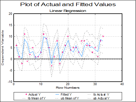
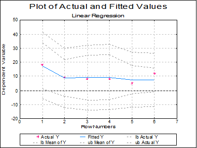
Plot of Actual and Fitted Values: Select this option to plot actual and fitted Y values and their confidence intervals against row numbers (index), residuals or against any independent variable. A further dialogue will enable you to choose the X-axis variable from a list containing Row Numbers, Residuals and all independent variables.
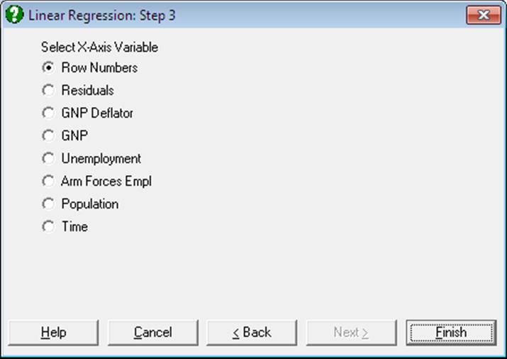
By default, a line graph of the two series is plotted. However, since this procedure (like the plot of residuals) uses the X-Y Plots engine, it has almost all controls and options available for X-Y Plots, except for error bars and right Y-axes. This means that, as well as being able to edit all aspects of the graph, you can connect data points with lines, curves or display confidence intervals.
The data points on the graph will also respond to the right mouse button in the way X-Y Plots does; the point is highlighted, a panel displays information about the point and in Stand-Alone Mode, the row of the spreadsheet containing the data point is also highlighted (a procedure which is also known as Brushing or Point identification). While the point is highlighted you can press <Delete> to omit the particular row containing the point. The entire Regression Analysis will be run again without the deleted row. If you want to restore the original regression, you will need to take one of the following two actions depending on the way you run UNISTAT:
1. In Stand-Alone Mode, go back to Data Processor and delete or deactivate the Select Row column created by the program.
2. In Excel Add-In Mode, highlight a different block of data to remove the effect of the internal Select Row column.
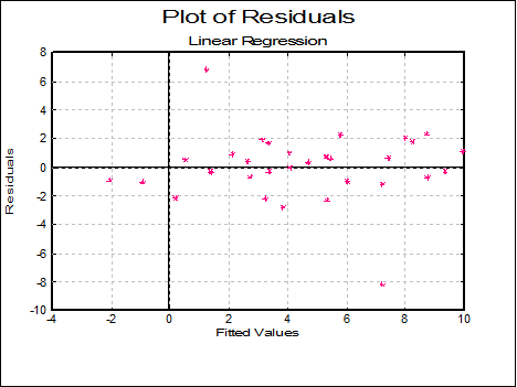
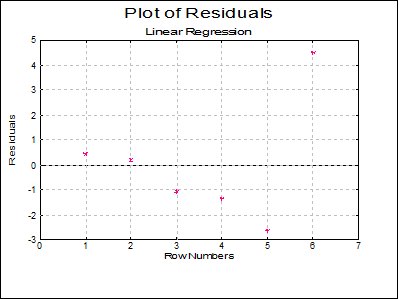
Plot of Residuals: Residuals can be plotted against row numbers (index), fitted values or against any independent variable. A further dialogue will enable you to choose the X-axis variable from a list containing Row Numbers, Fitted Values and all independent variables.
By default a scatter graph of residuals is plotted. For more information on available options see Plot of Actual and Fitted Values above.
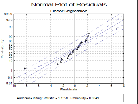
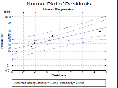
Normal Plot of Residuals: Residuals are plotted against the normal probability (probit) axis. For more information on available options see Plot of Actual and Fitted Values above (also see 5.3.2. Normal Probability Plot).
7.2.1.3. Linear Regression Examples
Example 1
Table 5.1 on p. 134 from Tabachnick, B. G. & L. S. Fidell (1989).
Open REGRESS, select Statistics 1 → Regression Analysis → Linear Regression and select Motiv, Qual and Grade (C6 to C8) as [Variable]s and Compr (C9) as [Dependent]. Select all output options to obtain the following results:
Linear Regression
Dependent Variable: Compr
Valid Number of Cases: 6, 0 Omitted
Regression Results
|
|
Coefficient |
Standard Error |
t-Statistic |
Probability |
Lower 95% |
Upper 95% |
|
Constant |
-4.7218 |
9.0656 |
-0.5208 |
0.6544 |
-43.7281 |
34.2845 |
|
Motiv |
0.6583 |
0.8721 |
0.7548 |
0.5292 |
-3.0942 |
4.4107 |
|
Qual |
0.2720 |
0.5891 |
0.4618 |
0.6896 |
-2.2627 |
2.8068 |
|
Grade |
0.4160 |
0.6462 |
0.6438 |
0.5857 |
-2.3643 |
3.1964 |
|
Residual Sum of Squares = |
30.3599 |
|
Standard Error = |
3.8961 |
|
Mean of Y = |
10.0000 |
|
Stand Dev of y = |
4.5166 |
|
Correlation Coefficient = |
0.8381 |
|
R-squared = |
0.7024 |
|
Adjusted R-squared = |
0.2559 |
|
F(3,2) = |
1.5731 |
|
Probability of F = |
0.4114 |
|
Durbin-Watson Statistic = |
1.7838 |
|
log of likelihood = |
-14.6736 |
|
Press Statistic = |
661.8681 |
ANOVA of Regression
|
Due To |
Sum of Squares |
DoF |
Mean Square |
F-Stat |
Prob |
|
Motiv |
35.042 |
1 |
35.042 |
2.308 |
0.2680 |
|
Qual |
30.306 |
1 |
30.306 |
1.996 |
0.2932 |
|
Grade |
6.292 |
1 |
6.292 |
0.415 |
0.5857 |
|
Regression |
71.640 |
3 |
23.880 |
1.573 |
0.4114 |
|
Error |
30.360 |
2 |
15.180 |
|
|
|
Total |
102.000 |
5 |
20.400 |
1.344 |
0.4787 |
Correlation Matrix of Regression Coefficients
|
|
Constant |
Motiv |
Qual |
Grade |
|
Constant |
1.0000 |
-0.8485 |
0.1286 |
-0.1935 |
|
Motiv |
-0.8485 |
1.0000 |
-0.1768 |
-0.1151 |
|
Qual |
0.1286 |
-0.1768 |
1.0000 |
-0.7455 |
|
Grade |
-0.1935 |
-0.1151 |
-0.7455 |
1.0000 |
Covariance Matrix of Regression Coefficients
|
|
Constant |
Motiv |
Qual |
Grade |
|
Constant |
82.1859 |
-6.7083 |
0.6870 |
-1.1338 |
|
Motiv |
-6.7083 |
0.7606 |
-0.0908 |
-0.0649 |
|
Qual |
0.6870 |
-0.0908 |
0.3471 |
-0.2838 |
|
Grade |
-1.1338 |
-0.0649 |
-0.2838 |
0.4176 |
Case (Diagnostic) Statistics
|
|
Actual Y |
Fitted Y |
95% lb Actual Y |
95% ub Actual Y |
95% lb Mean of Y |
95% ub Mean of Y |
Standard Error of Fitted |
|
1 |
18.0000 |
17.5675 |
-5.9769 |
41.1119 |
1.0353 |
34.0997 |
3.8423 |
|
2 |
9.0000 |
8.8399 |
-12.3120 |
29.9918 |
-4.0589 |
21.7387 |
2.9979 |
|
3 |
8.0000 |
9.0893 |
-13.9745 |
32.1531 |
-6.7510 |
24.9296 |
3.6815 |
|
4 |
8.0000 |
9.3562 |
-13.8431 |
32.5555 |
-6.6807 |
25.3932 |
3.7272 |
|
5 |
5.0000 |
7.6376 |
-11.9530 |
27.2281 |
-2.4997 |
17.7749 |
2.3561 |
|
6 |
12.0000 |
7.5095 |
-11.3204 |
26.3394 |
-1.0661 |
16.0851 |
1.9931 |
|
|
Standard ised Fitted |
Adjusted Fitted |
Residuals |
Standard Error of Residuals |
Standardised Residuals |
Studentised Residuals |
|
1 |
1.9992 |
2.2363 |
0.4325 |
0.6454 |
0.1110 |
0.6702 |
|
2 |
-0.3065 |
8.6076 |
0.1601 |
2.4885 |
0.0411 |
0.0643 |
|
3 |
-0.2406 |
18.1667 |
-1.0893 |
1.2753 |
-0.2796 |
-0.8541 |
|
4 |
-0.1701 |
23.9868 |
-1.3562 |
1.1348 |
-0.3481 |
-1.1951 |
|
5 |
-0.6241 |
9.1581 |
-2.6376 |
3.1031 |
-0.6770 |
-0.8500 |
|
6 |
-0.6580 |
5.9179 |
4.4905 |
3.3478 |
1.1525 |
1.3413 |
|
|
Press (Deleted) Residuals |
Studentised Press Residuals |
Leverage |
Cook’s Distance |
Mahalanobis Distance |
Welsch Distance |
|
1 |
15.7637 |
0.5382 |
0.8059 |
3.9802 |
4.0295 |
43.2522 |
|
2 |
0.3924 |
0.0455 |
0.4254 |
0.0015 |
2.1269 |
0.1920 |
|
3 |
-10.1667 |
-0.7578 |
0.7262 |
1.5199 |
3.6310 |
-14.9437 |
|
4 |
-15.9868 |
-1.5807 |
0.7485 |
3.8520 |
3.7425 |
-39.8563 |
|
5 |
-4.1581 |
-0.7520 |
0.1990 |
0.1041 |
0.9951 |
-1.6031 |
|
6 |
6.0821 |
2.9934 |
0.0950 |
0.1594 |
0.4751 |
4.6377 |
|
|
Covratio |
DfFit |
Standardised DfFit |
Delta-Beta Constant |
Delta-Beta Motiv |
Delta-Beta Qual |
|
1 |
210.8306 |
15.3312 |
3.2040 |
-20.9957 |
1.0201 |
0.6412 |
|
2 |
38.8964 |
0.2323 |
0.0549 |
0.1779 |
0.0036 |
0.0319 |
|
3 |
24.3153 |
-9.0774 |
-2.1875 |
-13.0714 |
1.6339 |
0.3631 |
|
4 |
1.2590 |
-14.6305 |
-5.1916 |
13.6116 |
-2.1874 |
1.6812 |
|
5 |
4.1991 |
-1.5205 |
-0.5710 |
-3.3462 |
0.1201 |
-0.1731 |
|
6 |
0.0022 |
1.5916 |
1.7821 |
3.8897 |
-0.1289 |
-0.1386 |
|
|
Delta-Beta Grade |
Standardised Delta-Beta Constant |
Standardised Delta-Beta Motiv |
Standardised Delta-Beta Qual |
Standardised Delta-Beta Grade |
|
1 |
0.5191 |
-1.8597 |
0.9392 |
0.8739 |
0.6451 |
|
2 |
-0.0421 |
0.0139 |
0.0029 |
0.0384 |
-0.0461 |
|
3 |
-0.9077 |
-1.2792 |
1.6622 |
0.5468 |
-1.2463 |
|
4 |
-0.8213 |
1.9858 |
-3.3171 |
3.7744 |
-1.6809 |
|
5 |
0.2728 |
-0.3266 |
0.1218 |
-0.2600 |
0.3735 |
|
6 |
-0.0043 |
0.9575 |
-0.3298 |
-0.5251 |
-0.0149 |
Example 2
Table 4.3.1 on p. 296 from Elliot, M. A., J. S. Reisch, N. P. Campbell (1989). This data set is known as Longley’s data and it is particularly sensitive to rounding-off errors and the regression algorithm used.
Open REGRESS, select Statistics 1 → Regression Analysis → Linear Regression and select GNP Deflator, GNP, Unemployment, Arm Forces Empl, Population and Time (C10 to C15) as [Variable]s and Total (C16) as [Dependent]. Select only the Regression Results output option to obtain the following:
Linear Regression
Dependent Variable: Total
Valid Number of Cases: 16, 0 Omitted
Regression Results
|
|
Coefficient |
Standard Error |
t-Statistic |
|
Constant |
-3482258.634596 |
890420.3836074 |
-3.910802918154 |
|
GNP Deflator |
15.06187227137 |
84.91492577477 |
0.17737602823 |
|
GNP |
-0.0358191792926 |
0.0334910077722 |
-1.069516317221 |
|
Unemployment |
-2.020229803817 |
0.488399681652 |
-4.136427355941 |
|
Arm Forces Empl |
-1.033226867174 |
0.214274163162 |
-4.821985310445 |
|
Population |
-0.0511041056536 |
0.226073200069 |
-0.226051144664 |
|
Time |
1829.151464614 |
455.4784991422 |
4.01588981271 |
|
|
Probability |
Lower 95% |
Upper 95% |
|
Constant |
0.0036 |
-5496534.8253 |
-1467982.4439 |
|
GNP Deflator |
0.8631 |
-177.0295 |
207.1533 |
|
GNP |
0.3127 |
-0.1116 |
0.0399 |
|
Unemployment |
0.0025 |
-3.1251 |
-0.9154 |
|
Arm Forces Empl |
0.0009 |
-1.5179 |
-0.5485 |
|
Population |
0.8262 |
-0.5625 |
0.4603 |
|
Time |
0.0030 |
798.7848 |
2859.5181 |
|
Residual Sum of Squares = |
836424.0555059 |
|
Standard Error = |
304.854073562 |
|
Mean of Y = |
65317 |
|
Stand Dev of y = |
3511.96835597 |
|
Correlation Coefficient = |
0.997736941572 |
|
R-squared = |
0.995479004577 |
|
Adjusted R-squared = |
0.992465007629 |
|
F(6,9) = |
330.2853392354 |
|
Probability of F = |
0.0000 |
|
Durbin-Watson Statistic = |
2.559487689283 |
|
log of likelihood = |
-110.7203479964 |
|
Press Statistic = |
2886892.562947 |
WARNING! Table 4.3.1 contains a misprint in row 13 of the (X5) variable. The above results have been obtained by using the correct value of 123366.
Example 3
Example 20.1c on p. 426 from Zar, J. H. (2010).
Open REGRESS, select Statistics 1 → Regression Analysis → Linear Regression and select temperature, cm, mm and min (C1 to C4) as [Variable]s and ml (C5) as [Dependent]. Select only the Regression Results and ANOVA of Regression output options to obtain the following results:
Linear Regression
Dependent Variable: ml
Valid Number of Cases: 33, 0 Omitted
Regression Results
|
|
Coefficient |
Standard Error |
t-Statistic |
Probability |
Lower 95% |
Upper 95% |
|
Constant |
2.9583 |
1.3636 |
2.1695 |
0.0387 |
0.1651 |
5.7515 |
|
temperature |
-0.1293 |
0.0213 |
-6.0751 |
0.0000 |
-0.1729 |
-0.0857 |
|
cm |
-0.0188 |
0.0563 |
-0.3338 |
0.7410 |
-0.1341 |
0.0965 |
|
mm |
-0.0462 |
0.2073 |
-0.2230 |
0.8252 |
-0.4708 |
0.3784 |
|
min |
0.2088 |
0.0670 |
3.1141 |
0.0042 |
0.0714 |
0.3461 |
|
Residual Sum of Squares = |
5.0299 |
|
Standard Error = |
0.4238 |
|
Mean of Y = |
2.4742 |
|
Stand Dev of y = |
0.6789 |
|
Correlation Coefficient = |
0.8117 |
|
R-squared = |
0.6589 |
|
Adjusted R-squared = |
0.6102 |
|
F(4,28) = |
13.5235 |
|
Probability of F = |
0.0000 |
|
Durbin-Watson Statistic = |
1.9947 |
|
log of likelihood = |
-15.9976 |
|
Press Statistic = |
7.1248 |
ANOVA of Regression
|
Due To |
Sum of Squares |
DoF |
Mean Square |
F-Stat |
Prob |
|
|
temperature |
7.876 |
1 |
7.876 |
43.845 |
0.0000 |
|
|
cm |
0.013 |
1 |
0.013 |
0.073 |
0.7888 |
|
|
mm |
0.086 |
1 |
0.086 |
0.478 |
0.4950 |
|
|
min |
1.742 |
1 |
1.742 |
9.698 |
0.0042 |
|
|
Regression |
9.717 |
4 |
2.429 |
13.524 |
0.0000 |
|
|
Error |
5.030 |
28 |
0.180 |
|
|
|
|
Total |
14.747 |
32 |
0.461 |
2.565 |
0.0066 |
|