7.2.2. Polynomial Regression
Polynomials can be fitted on multivariate data. There are no restrictions on the degree of polynomials, but you need to remember that with high degree polynomials number overflow problems may occur.
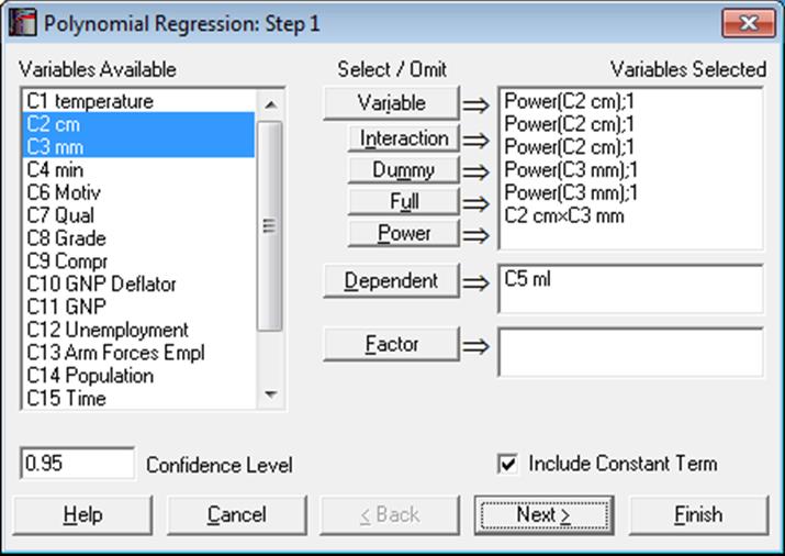
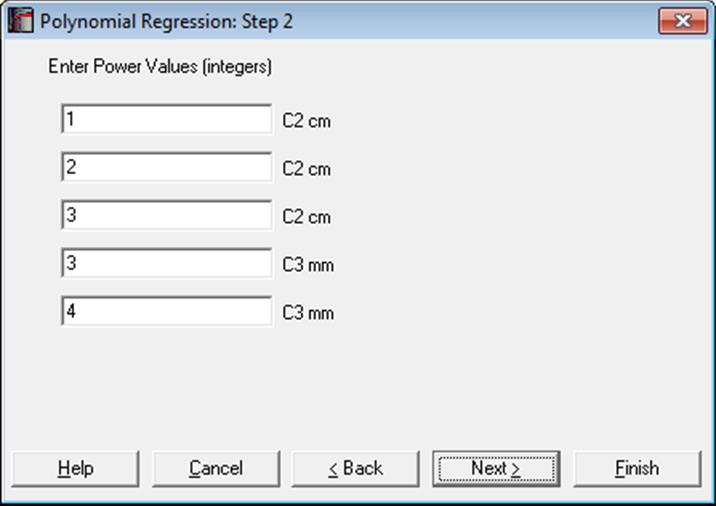
As in Linear Regression, it is possible to create interaction terms, dummy variables, select multiple dependent variables and run regressions on subsamples defined by several factor columns (see 7.2.1.1. Linear Regression Variable Selection). However, here, the Lag/Lead button is replaced with a Power button. Once you highlight a variable from the Variables Available list, you can create as many power terms for that variable as you wish, by clicking on the Power button. The power terms are created with a degree one. You can assign the desired powers on the next dialogue.
All output options available for the Linear Regression procedure will be available.
Fitted values for the Polynomial Regression are extremely sensitive to slight changes in coefficients. Therefore, use of the truncated coefficient values from the formatted output (as in text, Word or HTML) display is not recommended in reconstructing a fitted polynomial equation. To run predictions, you are advised to use the full precision Excel output or one of the two methods explained in section 7.2.1.2.2. Linear Regression Case Output. These functions use the full 16-digit precision of the estimated coefficients. The estimated coefficients will also be saved in full precision automatically in the file POLYCOEF.TXT, in the order they appear in the Regression Results output option.
Example 1
Open REGRESS, select Statistics 1 → Regression Analysis → Polynomial Regression. Highlight cm (C2) and click the Power button three times. Next, highlight mm (C3) and click the Power button twice. Then highlight both cm (C2) and mm (C3) and click the Interaction button once. Select ml (C5) as [Dependent]. On the Output Options Dialogue check only the Regression Results option.
Polynomial Regression
Dependent Variable: ml
Valid Number of Cases: 33, 0 Omitted
Regression Results
|
|
Coefficient |
Standard Error |
t-Statistic |
Probability |
Lower 95% |
Upper 95% |
|
Constant |
-46.8884 |
38.6993 |
-1.2116 |
0.2366 |
-126.4360 |
32.6592 |
|
cm^1 |
15.8446 |
12.3077 |
1.2874 |
0.2093 |
-9.4543 |
41.1436 |
|
cm^2 |
-1.5529 |
1.3422 |
-1.1570 |
0.2578 |
-4.3119 |
1.2060 |
|
cm^3 |
0.0539 |
0.0475 |
1.1341 |
0.2671 |
-0.0438 |
0.1515 |
|
mm^3 |
0.0464 |
0.1202 |
0.3856 |
0.7030 |
-0.2008 |
0.2935 |
|
mm^4 |
-0.0037 |
0.0132 |
-0.2795 |
0.7821 |
-0.0308 |
0.0234 |
|
cm x mm |
-0.2194 |
0.2598 |
-0.8445 |
0.4061 |
-0.7535 |
0.3147 |
|
Residual Sum of Squares = |
12.5474 |
|
Standard Error = |
0.6947 |
|
Mean of Y = |
2.4742 |
|
Standard Deviation of Y = |
0.6789 |
|
Correlation Coefficient = |
0.3862 |
|
R-squared = |
0.1492 |
|
Adjusted R-squared = |
-0.0472 |
|
F(6,26) = |
0.7597 |
|
Probability of F = |
0.6079 |
|
Durbin-Watson Statistic = |
1.9130 |
|
Log of Likelihood = |
-31.3034 |
|
Press Statistic = |
17.5842 |
Example 2
Table 4.4.1 on p. 295 from Elliot, M. A., J. S. Reisch, N. P. Campbell (1989). The following results are given on p. 297.
Open REGRESS, select Statistics 1 → Regression Analysis → Polynomial Regression and select X (C17) as [Variable] and Y (C18) as [Dependent]. The following set of outputs has been obtained by using these variables with only changing the degree of polynomial. Here we will only print the estimated regression coefficients:
Polynomial Regression
Dependent variable: Y
Valid Number of Cases: 19, 0 Omitted
Regression results
|
|
Coefficient |
standard error |
t-statistic |
Probability |
|
Constant |
37.3890 |
0.43640 |
85.6754 |
0.0000 |
|
X^1 |
3.12686 |
0.15099 |
20.7087 |
0.0000 |
|
|
Coefficient |
standard error |
t-statistic |
Probability |
|
Constant |
40.3017 |
1.13349 |
35.5554 |
0.0000 |
|
X^1 |
0.66658 |
0.91352 |
0.72968 |
0.4761 |
|
X^2 |
0.45397 |
0.16688 |
2.72031 |
0.0151 |
|
|
Coefficient |
standard error |
t-statistic |
Probability |
|
Constant |
32.7673 |
3.11320 |
10.5253 |
0.0000 |
|
X^1 |
10.4109 |
3.90298 |
2.66743 |
0.0176 |
|
X^2 |
-3.38682 |
1.51356 |
-2.23765 |
0.0408 |
|
X^3 |
0.47011 |
0.18442 |
2.54915 |
0.0222 |
|
|
Coefficient |
standard error |
t-statistic |
Probability |
|
Constant |
6.92654 |
7.28551 |
0.95073 |
0.3579 |
|
X^1 |
55.8348 |
12.4946 |
4.46873 |
0.0005 |
|
X^2 |
-31.4866 |
7.60544 |
-4.14001 |
0.0010 |
|
X^3 |
7.76246 |
1.95731 |
3.96587 |
0.0014 |
|
X^4 |
-0.67507 |
0.18076 |
-3.73460 |
0.0022 |
|
|
Coefficient |
standard error |
t-statistic |
Probability |
|
Constant |
36.2391 |
22.7989 |
1.58951 |
0.1360 |
|
X^1 |
-9.16153 |
49.5645 |
-0.18484 |
0.8562 |
|
X^2 |
23.3871 |
41.2381 |
0.56712 |
0.5803 |
|
X^3 |
-14.3460 |
16.4561 |
-0.87178 |
0.3991 |
|
X^4 |
3.59360 |
3.16090 |
1.13689 |
0.2761 |
|
X^5 |
-0.31740 |
0.23467 |
-1.35255 |
0.1993 |
|
|
Coefficient |
standard error |
t-statistic |
Probability |
|
Constant |
157.882 |
73.6834 |
2.14271 |
0.0533 |
|
X^1 |
-330.976 |
192.285 |
-1.72128 |
0.1109 |
|
X^2 |
364.043 |
201.286 |
1.80858 |
0.0956 |
|
X^3 |
-199.361 |
108.401 |
-1.83911 |
0.0908 |
|
X^4 |
58.1131 |
31.7588 |
1.82983 |
0.0922 |
|
X^5 |
-8.60699 |
4.81303 |
-1.78827 |
0.0990 |
|
X^6 |
0.50964 |
0.29560 |
1.72410 |
0.1103 |