9.4.4. Cox Regression
Apart from time and status variables, data for Survival Analysis often contain measurements on one or more continuous variables, such as temperature, dosage, age or one or more categorical variables such as gender, region, treatment. In such cases it is desirable to construct Life Tables (or survival functions) which reflect the effects of these continuous or categorical variables (which are also called covariates).
A method which combines the elements of nonparametric Life Table analysis and the parametric Regression Analysis was introduced by D R Cox in 1972. It is known as the Cox Regression or Cox’s proportional hazards model. The latter reflects a fundamental assumption of this model, namely that the hazard function of an individual in one group is proportional to the hazard function of another in another group at any time period. In graphical terms, this is equivalent to assuming that the hazard curves of different groups do not cross each other.
Let X be a matrix of p independent variables (covariates) for n cases. Then the hazard function for the jth case can be written as:
![]()
where:
· h0(t) is the baseline hazard function and
·
![]() is the vector of
coefficients.
is the vector of
coefficients.
Rearranging the terms we obtain:
![]()
Although the right-hand side of this equation is linear, the existence of another unknown on the left-hand side, h0(t), makes it impossible to solve it using the Linear Regression method. Instead, a maximum likelihood solution for a log-likelihood function that is derived from the above equation is found:
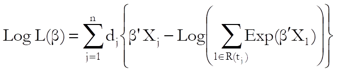
where R(tj) is the set of cases at risk at the start of time j and dj is the number of cases that terminate at time j.
The maximum likelihood solution of this proportional hazards model is computed employing a modified Newton-Raphson minimisation algorithm. The nature of this method implies that a solution (convergence) cannot always be achieved. In such cases, you are advised to edit the convergence parameters provided, in order to find the right levels for the particular problem at hand. Three convergence parameters can be edited in a dialogue that pops up just after the Variable Selection Dialogue (see 9.4.4.2. Cox Regression Intermediate Inputs).
Stratified Analysis: It may be the case that with some data sets the assumption of proportionality of individual hazard functions cannot be maintained. Under such circumstances it may be possible to define some subgroups within which the hazard functions can assumed to be proportional. This type of analysis is called a stratified analysis and the subgroups within which the proportionality assumption is maintained are called the strata.
The strata are defined by the levels of a factor column, which can be selected from the Variable Selection Dialogue. The program then assumes that different strata have different baseline hazard functions, but that they all have the same coefficient estimates for covariates. A maximum of six strata can be fitted simultaneously.
Baseline Functions at Means of Covariates: In order to maintain numerical stability, UNISTAT always centres the covariates by subtracting their respective means first. Most results, including the coefficient estimates, are invariant to centring. However, the baseline functions are different with and without centring and some sources prefer reporting the centred baseline functions while the others the uncentred ones (baseline functions relative to the origin). UNISTAT makes both sets of results available. See 9.4.4.2. Cox Regression Intermediate Inputs below for how to make this selection. The only other result that is affected by centring is the Linear Fit (XBeta) reported under Case (Diagnostic) Statistics (see 9.4.4.3.2. Cox Regression Further Output Options).
Predictions: If a case (row) of data does not contain any missing values except for the time variable, then a prediction of survival times is generated for this case. If at least one such case exists in data, then a fourth option Predicted Survival is added to the Baseline Functions dialogue. An additional column of predicted survival times is output for each predicted case.
9.4.4.1. Cox Regression Variable Selection
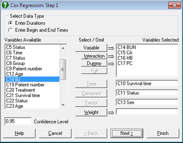
Variable: Any number of columns containing numeric data can be selected as independent variables (covariates). However, unlike any other regression procedures, a Cox regression can be run without selecting any independent variables. This is called the initial model (or the null model). UNISTAT reports the -2Log Likelihood value for the initial model for any model fitted.
Interaction: This button is used to create independent variables, which are the products of existing numeric variables. If only one variable is highlighted, then the new independent variable created will be the product of the selected column by itself. If two or more variables are highlighted, then the new term will be the product of these variables. Maximum three-way interactions are allowed. Interactions of dummy variables or lags are not allowed. In order to create interaction terms for dummy variables, create interactions first, and then create dummy variables for them. For further information see 2.1.4. Creating Interaction, Dummy and Lag/Lead Variables.
Dummy: This button is used to create n or n – 1 new independent (dummy or indicator) variables for a factor column containing n levels. Each dummy variable corresponds to a level of the factor column. A case in a dummy column will have the value of 1 if the factor contains the corresponding level in the same row, and 0 otherwise. If the selected variable is an interaction term, then dummy variables will be created for this interaction term. Up to three-way interactions are allowed and short or long string columns can be selected as factors. It is possible to include all n levels in the analysis or to omit the first or the last level to remove the inherent over-parameterisation of the model. For further information see 2.1.4. Creating Interaction, Dummy and Lag/Lead Variables.
Full: This button becomes activated when two or more categorical variables are highlighted. Like the [Dummy] button, it is also used to create dummy variables. The only difference is that this button will create all necessary dummy variables and their interactions to specify a complete model. For instance, if two categorical variables are highlighted, then this button will create two sets of dummy variables representing the main effects and a third set representing the interaction term. Maximum three-way interactions are supported.
Time: It is compulsory to select at least one column containing numeric data as the time variable. Two types of data can be selected for Cox Regression; (1) Enter Durations where one column is selected containing the duration of each case and (2) Enter Begin and End Times where one column is selected as the starting time and another column as the termination time. In the latter case, the program subtracts the second column from the first one to obtain the duration of each case. If this results in some non positive values, then they are treated as missing cases (see 3.0.2.4. Time Data).
Censored: This variable is selected to show whether the termination time of a case is not known or the termination event has occurred. If the value in the column is zero then it is assumed that the case has been censored, which means that it has been excluded from the study before the termination event has occurred. Non-zero values (usually one) indicate that the termination event has occurred for this case. If a censor variable is not selected, then it is assumed that termination event has occurred for all cases. The default value of 0 indicating the censored cases can be edited to any other value from the next dialogue (see 9.4.4.2. Cox Regression Intermediate Inputs).
Weight: A column containing continuous numeric data can be selected as a weight variable. In this case, the program will normalise this column so that its sum is equal to the valid number of cases and then multiply each covariate by its square root before running the regression.
Factor: A categorical variable containing a limited number of distinct values can be selected as a factor. Unlike other Survival Analysis procedures though, this variable is not used in selecting subgroups to be included in the analysis. All cases are included in the analysis, but a stratified model is fitted. For more information on stratified analysis see the beginning of section 9.4.4. Cox Regression.
9.4.4.2. Cox Regression Intermediate Inputs
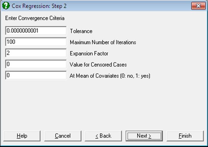
Tolerance: This value is used to control the sensitivity of nonlinear minimisation procedure employed. Under normal circumstances, you do not need to edit this value. If a convergence cannot be achieved, then larger values of this parameter can be tried by removing one or more zeros.
Maximum Number of Iterations: When convergence cannot be achieved with the default value of 100 function evaluations, a higher value can be tried.
Expansion Factor: When the nonlinear minimisation algorithm moves away from a valid range of input parameters, this expansion factor is used to start a new search in a wider area. Under normal circumstances, you do not need to edit this value. If convergence cannot be achieved, then other values of similar (but larger) magnitude can be tried.
Value for Censored Cases: If a column of the spreadsheet has been selected as a censor variable, UNISTAT will consider cases with a zero entry in this column as censored. However, you can specify any value here to indicate which cases are to be treated as censored. Once a change is made here, it will apply to all Survival Analysis procedures throughout the session.
At Mean of Covariates: This box is used to select the type of baseline survival and hazard functions. A zero value results in baseline functions being reported relative to the origin and other values relative to the covariate means.
One other result that is affected by this choice is the linear fit (XBeta) vector reported under the Case (Diagnostic) Statistics option.
Omit Level: This box will appear only when one or more dummy variables have been included in the model from the Variable Selection Dialogue. Three options are available; (0) do not omit any levels, (1) omit the first level and (2) omit the last level. When no levels are omitted, the model will usually be over-parameterised (see 2.1.4. Creating Interaction, Dummy and Lag/Lead Variables).
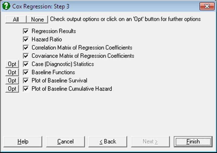
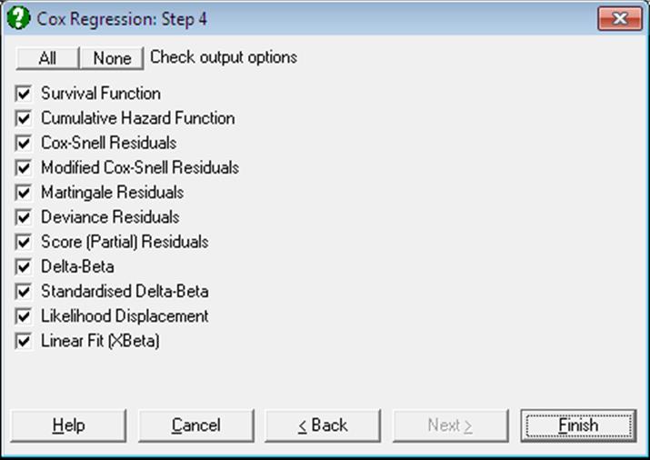
9.4.4.3. Cox Regression Output Options
When the maximum likelihood model has converged or the maximum number of iterations has been reached without convergence, an Output Options Dialogue will provide access to the following options.
When no covariates have been included in the model, only the -2 Log likelihood value will be reported in the Regression Results output. In this case, a Life Table will be displayed with a survival function that is identical to the Kaplan-Meier estimate of the same model (see 9.4.2. Kaplan-Meier Analysis).
9.4.4.3.1. Cox Regression Coefficient Output
Regression Results: The main regression output displays a table for coefficients of the estimated regression equation, their standard errors, Wald statistics, probability values and confidence intervals for the significance level specified in the Variable Selection Dialogue. If any independent variables have been omitted due to multicollinearity, they are reported at the end of the table. If you do not wish to display these variables enter the following line in the [Options] section of Documents\Unistat10\Unistat10.ini file:
DispCollin=0
In Stand-Alone Mode, the estimated regression coefficients can be saved to the data matrix by clicking on the UNISTAT icon situated on the Output Medium Toolbar.
Wald Statistic: This is defined as:
![]()
and has a chi-square distribution with one degree of freedom.
Confidence Intervals: The confidence intervals for regression coefficients are computed from:
![]()
where each coefficient’s standard error, ![]() , is the square root of the diagonal
element of covariance matrix.
, is the square root of the diagonal
element of covariance matrix.
-2 Log-Likelihood Initial Model: This is the value when all independent variables are excluded from the model:
![]()
-2 Log-Likelihood Final Model: This is -2 times the value of the log likelihood function when convergence is achieved.
Pseudo R-squared: In Cox Regression, an r-squared statistic as in the OLS regression is not available. This is because Cox Regression employs an iterative maximum likelihood estimation method. Equivalent statistics to test the goodness of fit have been proposed using the initial (L0) and maximum (L1) likelihood values.
McFadden:
![]()
Adjusted McFadden:
![]()
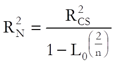
Cox & Snell:
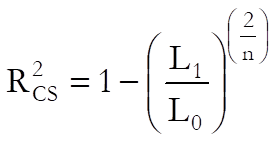
Nagelkerke:
Likelihood Ratio: This is a test statistic for the null hypothesis that “all regression coefficients for covariates are zero”. It is equal to -2 times the difference between the initial and final model likelihood values and has a chi-square distribution with k degrees of freedom (the number of independent variables in the model).
If no covariates have been included in the model, then only the -2 Log likelihood value will be reported.
Hazard Ratio:
Hazard ratio is defined as:
![]()
Values of hazard ratio above 1 indicate an increased hazard as the values of the corresponding covariate increase at any time period, and vice versa for values below 1.
The standard error of the hazard ratio is found as:
![]()
and its confidence intervals as:
![]()
which are simply the exponential of the coefficient confidence intervals.
This option is not available when no covariates have been included in the model.
Correlation Matrix of Regression Coefficients: This is a symmetric matrix with unity diagonal elements. The off-diagonal elements give the correlations between the regression coefficients.
This output is not available when no covariates have been included in the model.
Covariance Matrix of Regression Coefficients: This is a symmetric matrix where diagonal elements are the square of parameter standard errors.
This output is not available when no covariates have been included in the model.
9.4.4.3.2. Cox Regression Case Output
Case (Diagnostic) Statistics: Case statistics are useful in determining the influence of individual observations on the overall fit of the model. For further information see 7.2.1.2.2. Linear Regression Case Output.
The values reported here are not sorted according to strata and the time variable. Therefore, when this output is sent to the Data Processor for further analysis, a case-by-case correspondence with the original data will be maintained.
Survival Function:
![]()
Cumulative Hazard Function:
![]()
Cox-Snell Residuals:
![]()
These are identical to the cumulative hazard function.
Modified Cox-Snell Residuals:
![]()
where ![]() is if the
case terminates at time j and
is if the
case terminates at time j and ![]() if it is
censored.
if it is
censored.
Martingale Residuals:
![]()
Deviance Residuals:
![]()
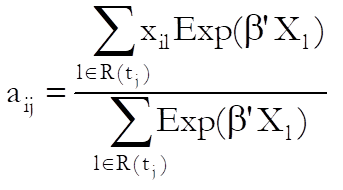
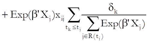
Score (Partial) Residuals:
![]() for
uncensored cases and missing otherwise for all covariates i = 1,…,p, where:
for
uncensored cases and missing otherwise for all covariates i = 1,…,p, where:
Delta-Beta:
![]() where
where ![]() is the p x p covariance matrix of regression coefficients and
is the p x p covariance matrix of regression coefficients and ![]() is an n x
p matrix, elements of which are defined as:
is an n x
p matrix, elements of which are defined as:
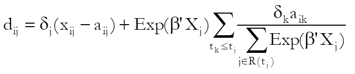
for j = 1,…,n, i = 1,…, p where ![]() is defined as in score residuals above.
is defined as in score residuals above.
Delta-beta is defined as the change in an estimated coefficient when a case is omitted from the analysis. However, unlike in Linear Regression (see 7.2.1.2.2. Linear Regression Case Output), where an exact estimate can be computed without having to run n regressions, the method employed here is an approximation (see Pettitt & Bin Daud, 1989). The user must be aware that different sources and statistical packages may adopt different approximation methods. The best way to find out which method gives the most accurate results is to run a small example and compute each delta-beta by running n regressions, each time omitting one row from the analysis.
Standardised Delta-Beta:
![]() for
i = 1,…, p.
for
i = 1,…, p.
This is delta-beta divided by its standard error for each coefficient.
Likelihood Displacement:
![]() where
where ![]() is the m x m covariance matrix of regression coefficients and
is the m x m covariance matrix of regression coefficients and ![]() is an n x
m matrix, elements of which are as defined in delta-betas. This statistic reflects the effect of deleting a case on the likelihood function.
is an n x
m matrix, elements of which are as defined in delta-betas. This statistic reflects the effect of deleting a case on the likelihood function.
Linear Fit (XBeta):
Defined as:
![]()
Alongside baseline functions, this is the only result that is affected by whether the baseline functions are reported centred or relative to the origin (see 9.4.4.2. Cox Regression Intermediate Inputs).
Baseline Functions: Baseline survival, hazard and cumulative hazard functions are reported for each stratum, which are ordered according to the time variable in ascending order. Baseline functions reported here would in general be different for a model where the covariates are centred. If there are no predicted cases, then the Baseline Functions dialogue contains three options.
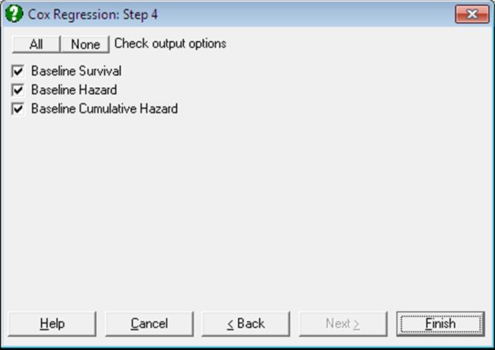
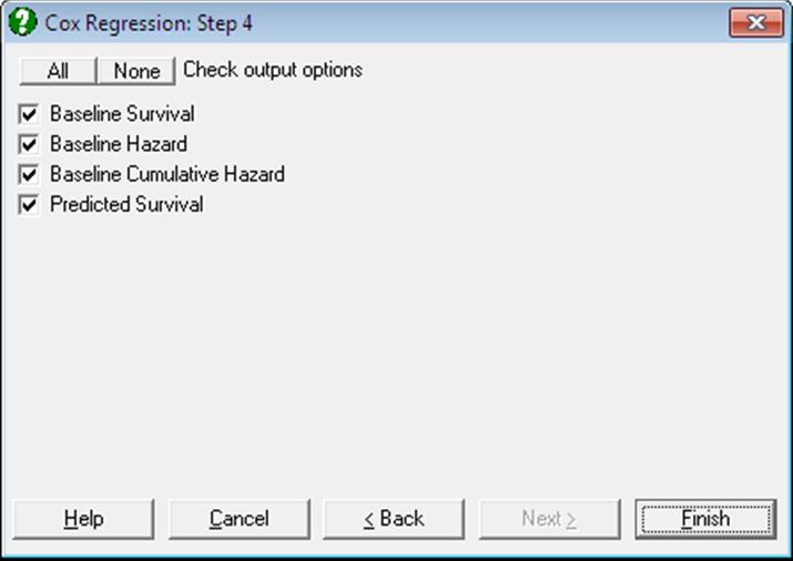
If at least one case (row) of data does not contain any missing values except for the time variable, then a fourth option Predicted Survival is added to the Baseline Functions dialogue.
Baseline Survival:
![]()
where ![]() is
obtained by solving the following equation:
is
obtained by solving the following equation:
![]()
where D(tj) is the set of cases that terminate at time j.
Baseline Hazard:
![]()
where ![]() is as
defined for the baseline survival.
is as
defined for the baseline survival.
Baseline Cumulative Hazard:
![]()
Predicted Survival: This is computed for cases containing no missing values except for the time variable. For each such case, a column of predicted survival times is computed as:
![]()
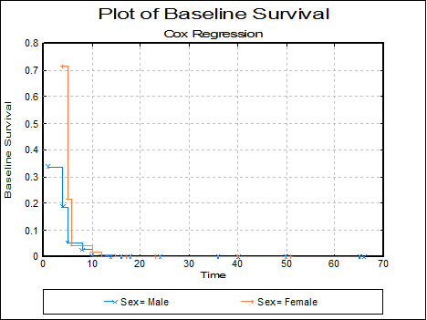
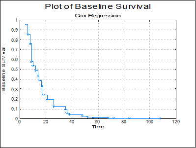
Plot of Baseline Survival Function: The baseline survival function is plotted against time. The appearance of this graph depends on the selection of estimation at covariate means (see 9.4.4.2. Cox Regression Intermediate Inputs).
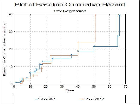
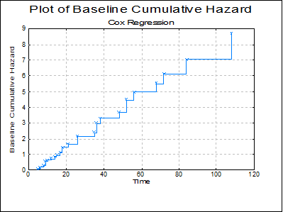
Plot of Baseline Cumulative Hazard: The baseline cumulative hazard function is plotted against time. The appearance of this graph depends on the selection of estimation method, at origin or at covariate means (see 9.4.4.2. Cox Regression Intermediate Inputs).
9.4.4.4. Cox Regression Examples
Example 1
Data on survival times of patients in a study on multiple myeloma is given in Table 1.3 (p. 9), in Collett, D. (1994).
Open SURVIVAL and select Statistics 2 → Survival Analysis → Cox Regression. From the Variable Selection Dialogue select the data option 1 Enter Durations and Survival time (C10) as [Time], Status (C11) as [Censored] and Age, Sex, BUN, CA, HB, PC and BJ (C12 to C18) as [Variable]s.
The Regression Results output reproduces the coefficient estimates and their standard errors as Collett reports them on Table 3.1 (p. 71):
Cox Regression
Time Variable: Survival time
Censor Variable: Status
Number of Cases Censored: 12 ( 25.0%)
Valid Number of Cases: 48, 0 Omitted
Regression Results
|
|
Coefficient |
Standard Error |
Wald statistic |
Probability |
Lower 95% |
Upper 95% |
|
Age |
-0.0194 |
0.0279 |
0.4806 |
0.4882 |
-0.0741 |
0.0354 |
|
Sex |
-0.2509 |
0.4023 |
0.3890 |
0.5328 |
-1.0394 |
0.5376 |
|
BUN |
0.0208 |
0.0059 |
12.3396 |
0.0004 |
0.0092 |
0.0324 |
|
CA |
0.0131 |
0.1324 |
0.0098 |
0.9211 |
-0.2465 |
0.2727 |
|
HB |
-0.1352 |
0.0689 |
3.8537 |
0.0496 |
-0.2703 |
-0.0002 |
|
PC |
-0.0016 |
0.0066 |
0.0587 |
0.8085 |
-0.0145 |
0.0113 |
|
BJ |
-0.6404 |
0.4267 |
2.2529 |
0.1334 |
-1.4767 |
0.1959 |
|
-2 Log likelihood: |
|
|
Initial Model = |
215.9399 |
|
Final Model = |
199.7009 |
|
Pseudo R-squared: |
|
|
McFadden = |
0.0752 |
|
Adjusted McFadden = |
0.0104 |
|
Cox & Snell = |
0.2870 |
|
Nagelkerke = |
0.2903 |
|
Likelihood Ratio Statistic: |
|
|
Chi-Square Statistic = |
16.2390 |
|
Degrees of Freedom = |
7 |
|
Right-Tail Probability = |
0.0230 |
Example 2
Survival times of patients classified according to age group and whether or not they have had a nephrectomy is given in Table 3.3 (p. 76), in Collett, D. (1994). Example 3.2 (p. 69).
Open SURVIVAL and select Statistics 2 → Survival Analysis → Cox Regression. From the Variable Selection Dialogue select the data option 1 Enter Durations and Time (C27) as [Time], Status (C28) as [Censored]. Then highlight Age group (C30) and click [Dummy] then highlight Nephrectomy (C29) and click [Dummy] again. This will add two terms to the model: Dummy(C30 Age Group) and Dummy(C29 Nephrectomy). The next dialogue will ask for a number of model parameters. Leave all entries unchanged as suggested by the program, but change the last one Omit Level? from 0 to 1, to omit the first level of each factor from the model.
The Regression Results output reproduces the coefficient estimates and their standard errors as Collett reports them in Example 3.12 (p. 100):
Cox Regression
Time Variable: Time
Censor Variable: Status
Number of Cases Censored: 4 ( 11.1%)
Valid Number of Cases: 36, 0 Omitted
Regression Results
|
|
Coefficient |
Standard Error |
Wald Statistic |
Signifi cance |
Lower 95% |
Upper 95% |
|
Age Group = 2 |
0.0125 |
0.4246 |
0.0009 |
0.9765 |
-0.8197 |
0.8447 |
|
3 |
1.3416 |
0.5918 |
5.1396 |
0.0234 |
0.1817 |
2.5014 |
|
Nephrectomy = 2 |
-1.4115 |
0.5152 |
7.5044 |
0.0062 |
-2.4213 |
-0.4016 |
|
-2 Log likelihood: |
|
|
Initial Model = |
177.6665 |
|
Final Model = |
165.5084 |
|
Pseudo R-squared: |
|
|
McFadden = |
0.0684 |
|
Adjusted McFadden = |
0.0347 |
|
Cox & Snell = |
0.2866 |
|
Nagelkerke = |
0.2887 |
|
Likelihood Ratio Statistic: |
|
|
Chi-Square Statistic = |
12.1581 |
|
Degrees of Freedom = |
3 |
|
Right-Tail Probability = |
0.0069 |
Hazard Ratio
|
|
Hazard Ratio |
Standard Error |
Lower 95% |
Upper 95% |
|
Age Group = 2 |
1.0126 |
0.4299 |
0.4406 |
2.3273 |
|
3 |
3.8250 |
2.2635 |
1.1993 |
12.1996 |
|
Nephrectomy = 2 |
0.2438 |
0.1256 |
0.0888 |
0.6692 |
Correlation Matrix of Regression Coefficients
|
|
Age Group = 2 |
3 |
Nephrectomy = 2 |
|
Age Group = 2 |
1.0000 |
0.3119 |
0.0767 |
|
3 |
0.3119 |
1.0000 |
0.0818 |
|
Nephrectomy = 2 |
0.0767 |
0.0818 |
1.0000 |
The baseline functions are reported as in Collett Table 3.10 (p. 101):
Cox Regression
Baseline Functions
|
Time |
Baseline Survival |
Baseline Hazard |
Baseline Cumulative Hazard |
|
5 |
0.9502 |
0.0498 |
0.0510 |
|
6 |
0.8516 |
0.1038 |
0.1607 |
|
8 |
0.7552 |
0.1132 |
0.2808 |
|
9 |
0.5761 |
0.2371 |
0.5514 |
|
10 |
0.5339 |
0.0733 |
0.6275 |
|
12 |
0.4861 |
0.0896 |
0.7214 |
|
14 |
0.4335 |
0.1082 |
0.8359 |
|
15 |
0.3831 |
0.1163 |
0.9595 |
|
17 |
0.3326 |
0.1318 |
1.1008 |
|
18 |
0.2379 |
0.2848 |
1.4360 |
|
21 |
0.1939 |
0.1851 |
1.6406 |
|
26 |
0.1198 |
0.3822 |
2.1222 |
|
35 |
0.0920 |
0.2319 |
2.3860 |
|
36 |
0.0512 |
0.4430 |
2.9712 |
|
38 |
0.0369 |
0.2792 |
3.2985 |
|
48 |
0.0259 |
0.2993 |
3.6543 |
|
52 |
0.0114 |
0.5598 |
4.4748 |
|
56 |
0.0070 |
0.3823 |
4.9565 |
|
68 |
0.0041 |
0.4207 |
5.5024 |
|
72 |
0.0022 |
0.4673 |
6.1323 |
|
84 |
0.0009 |
0.5975 |
7.0424 |
|
108 |
0.0002 |
0.8072 |
8.6886 |
Example 3
Data on times to removal of a catheter following a kidney infection is given in Table 5.1 (p. 157), in Collett, D. (1994), Example 3.2 (p. 69).
Open SURVIVAL and select Statistics 2 → Survival Analysis → Cox Regression. From the Variable Selection Dialogue select the data option 1 Enter Durations and Time (C32) as [Time], Status (C33) as [Censored]. Then select Age (C34) and Sex (C35) as [Variable]s. From the Output Options Dialogue select Case (Diagnostic) Statistics and at the next dialogue click All to select all options.
Different types of residuals calculated are reported by Collett in Table 5.2 (p. 157). Collett also reports the approximate estimated delta-betas in Table 5.4 (p. 172) and the likelihood displacement values in Table 5.5 (p.176).
Cox Regression
Case (Diagnostic) Statistics
|
Row |
Survival Function |
Cumulative Hazard Function |
Cox-Snell Residuals |
Modified Cox-Snell Residuals |
Martingale Residuals |
Deviance Residuals |
|
1 |
0.7200 |
0.3286 |
0.3286 |
0.3286 |
0.6714 |
0.9398 |
|
2 |
0.9245 |
0.0785 |
0.0785 |
0.0785 |
0.9215 |
1.8020 |
|
3 |
0.2386 |
1.4331 |
1.4331 |
1.4331 |
-0.4331 |
-0.3828 |
|
4 |
0.9104 |
0.0939 |
0.0939 |
0.0939 |
0.9061 |
1.7087 |
|
5 |
0.1697 |
1.7736 |
1.7736 |
1.7736 |
-0.7736 |
-0.6334 |
|
6 |
0.7322 |
0.3117 |
0.3117 |
1.3117 |
-0.3117 |
-0.7895 |
|
7 |
0.7668 |
0.2655 |
0.2655 |
0.2655 |
0.7345 |
1.0877 |
|
8 |
0.5836 |
0.5386 |
0.5386 |
0.5386 |
0.4614 |
0.5611 |
|
9 |
0.1916 |
1.6523 |
1.6523 |
1.6523 |
-0.6523 |
-0.5480 |
|
10 |
0.2409 |
1.4234 |
1.4234 |
1.4234 |
-0.4234 |
-0.3751 |
|
11 |
0.2415 |
1.4207 |
1.4207 |
1.4207 |
-0.4207 |
-0.3730 |
|
12 |
0.0914 |
2.3927 |
2.3927 |
2.3927 |
-1.3927 |
-1.0201 |
|
… |
… |
… |
… |
… |
… |
… |
|
Row |
Score (Partial) Residuals Age |
Score (Partial) Residuals Sex |
Delta-Beta Age |
Delta-Beta Sex |
Standardised Delta-Beta Age |
Standardised Delta-Beta Sex |
|
1 |
-1.0850 |
-0.2416 |
0.0020 |
-0.1977 |
0.0750 |
-0.1804 |
|
2 |
14.4930 |
0.6644 |
0.0004 |
0.5433 |
0.0155 |
0.4957 |
|
3 |
3.1291 |
-0.3065 |
-0.0011 |
0.0741 |
-0.0402 |
0.0677 |
|
4 |
-10.2215 |
0.4341 |
-0.0119 |
0.5943 |
-0.4528 |
0.5423 |
|
5 |
-16.5882 |
-0.5504 |
0.0049 |
0.0139 |
0.1869 |
0.0127 |
|
6 |
* |
* |
-0.0005 |
-0.1192 |
-0.0206 |
-0.1088 |
|
7 |
-17.8286 |
-0.0000 |
-0.0095 |
0.1269 |
-0.3607 |
0.1158 |
|
8 |
-7.6201 |
-0.0000 |
-0.0032 |
-0.0346 |
-0.1235 |
-0.0315 |
|
9 |
17.0910 |
-0.0000 |
-0.0073 |
-0.0733 |
-0.2771 |
-0.0669 |
|
10 |
10.2390 |
-0.0000 |
0.0032 |
-0.2023 |
0.1232 |
-0.1846 |
|
11 |
2.8575 |
-0.0000 |
0.0060 |
-0.2158 |
0.2279 |
-0.1970 |
|
12 |
5.5338 |
-0.0000 |
0.0048 |
-0.1939 |
0.1829 |
-0.1770 |
|
… |
… |
… |
… |
… |
… |
… |
|
Row |
Likelihood Displacement |
Linear Fit (XBeta) |
|
1 |
0.0328 |
-1.8604 |
|
2 |
0.3387 |
-4.0852 |
|
3 |
0.0046 |
-1.7389 |
|
… |
… |
… |
|
9 |
0.1334 |
-3.5993 |
|
10 |
0.0353 |
-4.1156 |
|
11 |
0.0611 |
-4.5104 |
|
12 |
0.0432 |
-4.4800 |
|
… |
… |
… |