9.4.3. Survival Comparison Statistics

Survival comparison tests are nonparametric rank tests and they are used to test the equality of survival functions for different groups defined by a factor column. Therefore, unlike other survival procedures, the choice of a factor column is compulsory here. It is also possible to select a weights variable for a weighted analysis.

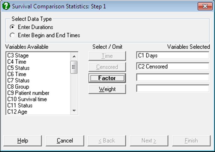
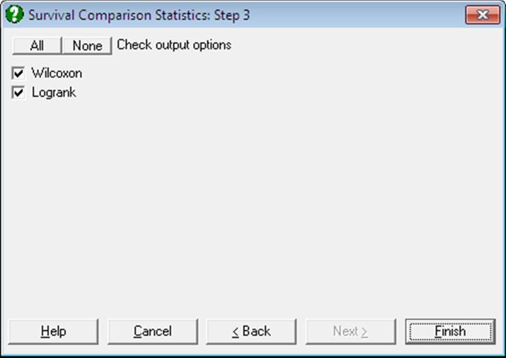
Once the data has been selected (see 9.4.0. Survival Analysis Variable Selection) a dialogue will appear facilitating selection of factor levels to be compared. Any number of levels can be selected. UNISTAT will then display an Output Options Dialogue featuring Wilcoxon and Logrank options.

9.4.3.1. Wilcoxon Tests: Gehan (Lee Desu), Breslow

This test is appropriate when the hazard functions are not necessarily proportional. The null hypothesis that “the groups do not differ” is tested.

First, all cases from all groups, censored or uncensored, are sorted according to survival times in ascending order. For each unique time period which is not censored, the number of deaths and the number of survivors (including the current time period), censored or uncensored, are computed. For tied time periods containing at least one censored subject, the same entities are also computed. For each time period, the expected value of deaths and its variance are computed and their sum is stored over all time periods, which are then used to compute the test statistic, which is approximately chi-square distributed.

Let us first consider a 2-group case to illustrate the Breslow algorithm. This is more robust than the older Gehan (Lee-Desu) method. Let:

·        d_jA = deaths in group A at time j, t_j,

·        d_j = deaths in all groups at time j,

·        n_jA = subjects alive in group A just before t_j,

·        n_j = subjects alive in all groups just before t_j,

·        N = total number of cases

For each time period j we can construct the following table:

 

	Died	Survived	Total
Group A	djA	njA - djA	njA
Group B	djB	njB - djB	njB
Total	dj	nj - dj	nj

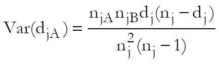
The difference between observed and expected value of deaths, weighted by the total number of individuals at risk, is computed for each time period:

  

Expected value of the variance is:

  

Summing over all time periods we obtain scores for each group:

  

and the overall variance:

  

Then the test statistic is computed as:

  

which has r - 1 degrees of freedom, where r is the number of groups (r = 2 and degrees of freedom = 1 in this case). UNISTAT uses an r-group generalisation of this algorithm.

The Gehan (Lee-Desu) statistic also requires computing the individual scores at each time period as follows:

For a censored case at time j:

   U_j = Unc_j

and for an uncensored case:

   U_j = 2 * Unc_j - UncEq_j + Cen_j - CenEq_j - N

where UncEq_j and CenEq_j are the number of uncensored and censored cases at each time period and Unc_j and Cen_j are the number of uncensored and censored cases at all current and previous time periods.

The test statistic is given as:

  

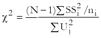
where SS_i is the sum of scores for group i.

9.4.3.2. Logrank Test: Mantel-Haenszel (Peto)

This test is appropriate when the hazard functions are proportional. The null hypothesis that “the groups do not differ” is tested. It is analogous to Mantel-Haenszel test for contingency tables.

As in Wilcoxon test (see 9.4.3.1. Wilcoxon Tests: Gehan (Lee Desu), Breslow), a 2 x 2 table is constructed for each time period. Then the expected value of deaths and its variance are computed as:

  

  

and then they are summed over all periods:

  

  

  

The test statistic is computed as:

  

which has r - 1 degrees of freedom, where r is the number of groups (r = 2 and degrees of freedom = 1 in this case). UNISTAT uses an r‑group generalisation of this algorithm.

9.4.3.3. Survival Comparison Tests Examples

Example 1

Example 14.1 on p. 479 from Armitage, P. & G. Berry (1994). Data on survival of patients with diffuse hystiocytic lymphoma according to stage of tumour are given.

Open SURVIVAL and select Statistics 2 → Survival Analysis → Survival Comparison Statistics. From the Variable Selection Dialogue select the data option 1 Enter Durations and Days (C1) as [Time], Censored (C2) as [Censored] and Stage (C3) as [Factor]. Include both factor levels 3 and 4 and check both output options to obtain the following results:

Survival Comparison Statistics

Wilcoxon

Stage	Total	Died	Censored	% Censored	Score	Mean Score
3	19	8	11	57.89%	-396	-20.8421
4	61	46	15	24.59%	396	6.4918
Total	80	54	26	32.50%	0

 

Gehan (Lee-Desu):
Chi-Square Statistic =	5.5428
Degrees of Freedom =	1
Right-Tail Probability =	0.0186
Breslow:
Chi-Square Statistic =	5.0998
Degrees of Freedom =	1
Right-Tail Probability =	0.0239

 

Logrank

Stage	Total	Observed	Expected	(O-E)^2/E	(O-E)^2/V
3	19	8	16.6870	4.5223	6.7097
4	61	46	37.3130	2.0225	6.7097
Total	80	54	54.0000	6.5448

 

Mantel-Haenszel (Peto):
Chi-Square Statistic =	6.7097
Degrees of Freedom =	1
Right-Tail Probability =	0.0096

 

Example 2

Data on survival times of women with tumours which were negatively or positively stained with PHA is given in Table 1.2 (p. 7), in Collett, D. (1994). Examples 2.11 (p. 40) and 2.12 (p. 44) give the results of Logrank and Wilcoxon tests respectively.

Open SURVIVAL and select Statistics 2 → Survival Analysis → Survival Comparison Statistics. From the Variable Selection Dialogue select the data option 1 Enter Durations and time (C6) as [Time], status (C7) as [Censored] and group (C8) as [Factor]. Include both factor levels 1 and 2 and check both output options to obtain the following results:

Survival Comparison Statistics

Wilcoxon

Group	Total	Died	Censored	% Censored	Score	Mean Score
0	32	21	11	34.38%	159	4.9688
1	13	5	8	61.54%	-159	-12.2308
Total	45	26	19	42.22%	0

 

Gehan (Lee-Desu):
Chi-Square Statistic =	4.5420
Degrees of Freedom =	1
Right-Tail Probability =	0.0331
Breslow:
Chi-Square Statistic =	4.1800
Degrees of Freedom =	1
Right-Tail Probability =	0.0409

 

Logrank

Group	Total	Observed	Expected	(O-E)^2/E	(O-E)^2/V
0	32	21	16.4349	1.2681	3.5150
1	13	5	9.5651	2.1788	3.5150
Total	45	26	26.0000	3.4468

 

Mantel-Haenszel (Peto):
Chi-Square Statistic =	3.5150
Degrees of Freedom =	1
Right-Tail Probability =	0.0608