9.4.2. Kaplan-Meier Analysis

The main difference between Life Table and Kaplan-Meier Analysis is that while cases are aggregated into time intervals in the former, the latter estimates the survival function on individual cases without any aggregation. The Kaplan-Meier estimate of the survival function is given by:

    

where:

·        d_j = number of deaths at interval j, and

·        n_j = number of cases entering interval j.

This is similar to the Life Table estimate of the survival function except that the number of cases entering interval j here replaces the average at risk in Life Table.

Variables are selected as described at the beginning of this chapter (see 9.4.0. Survival Analysis Variable Selection). If a factor variable has been selected, then a further dialogue will allow levels of the factor to be selected for analysis.

The Output Options Dialogue will provide access to the following four options:

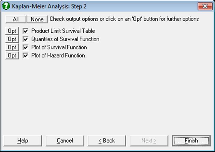
9.4.2.1. Product Limit Survival Table

The Kaplan-Meier estimate of the survival function is also called the product limit estimator. The Kaplan-Meier Analysis has the advantage over Life Table analysis in that its results do not depend on grouping of the data into intervals. The product limit method is like a Life Table with a single observation in each interval.

The survival and hazard functions are estimated and they are displayed together with their standard errors and confidence intervals for a user-defined confidence level.

Status: This indicates whether a case is censored. By default, 0 is censored (the termination time is not known) and non-zero values are uncensored (terminating at this time period).

Number Entering:

n_j: The number of cases that enter the interval.

Number Terminating:

d_j: The number terminating is the number of cases that reach the terminal event within the interval.

Cumulative Proportion Surviving:

     

The cumulative proportion surviving is the proportion of cases that have not reached the terminal event by the end of the interval.

Standard Error of Cumulative Surviving:

     

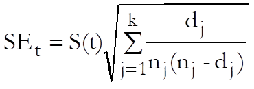
The standard error of cumulative proportion surviving is computed from Greenwood’s formula.

Confidence Intervals of Cumulative Surviving:

     

where the log-transformed standard error is:

     

SE_t (the standard error reported in the table) is not used in computing the confidence intervals, employing the standard Z distribution, because it often leads to values outside the valid range of 0 to 1. The significance level can be set to any value between 0 and 1 from the Variable Selection Dialogue.

Cumulative Proportion Terminating:

1-S(t): This is the cumulative proportion of cases that have reached the terminal event by the end of the interval and it is equal to one minus cumulative proportion surviving.

Standard Error of Cumulative Terminating:

SE_t: This is identical to the standard error of cumulative proportion surviving.

Confidence Intervals of Cumulative Terminating:

     

This is equal to one minus confidence intervals of surviving.

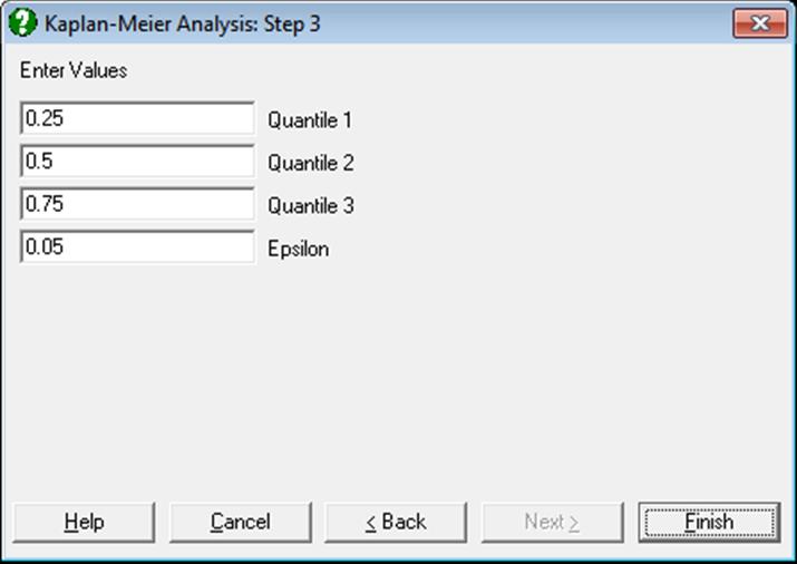
9.4.2.2. Quantiles of Survival Function

With this procedure it is possible to estimate the mean and up to three quantiles of the survival function. The quantiles are set to quartiles by default, but you can edit these to any values between 0 and 1. The value of epsilon (0.05 by default), which is used in estimating the standard error of quantiles, can also be changed. The mean and quantiles, as well as their standard errors and confidence intervals, are displayed in a table.

The mean survival time is computed as:

  

and its standard error is:

  

where:

  

and d is the total number of cases terminating.

The quantile 100p (where p = 0.5 is the median) of the survival function is given as the minimum observed survival time for which the value of the survival function is less than or equal to p. That is:

  

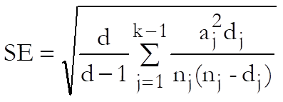
The standard error of a quantile is calculated from:

  

where

    = the standard error of survival function at t(p),

  

and:

  

  

Although the default value for epsilon is 0.05, you can enter any value between 0 and 1.

9.4.2.3. Kaplan-Meier Plots

Survival and hazard functions can be plotted. The Edit → Data Series dialogue provides the necessary controls to edit all aspects of the plot. If a factor column is selected, each subgroup’s settings are controlled from a different tab on the same dialogue. There are no limitations on the maximum number of subgroups that can be plotted on one graph, but only the properties of the first nine subgroups can be controlled from the Edit → Data Series dialogue.

The line type is set to Step Right by default (see 4.1.1.1.1. Line), following Armitage & Berry (1994) and Altman (1991). But this can be changed to Step Down following Collett (1994) from the Edit → Data Series → Line dialogue.

It is possible to display standard errors or confidence intervals for each subgroup separately. To do this, first display the graph and then select Edit → Data Series. Clicking on the [Bars…] button, a small dialogue will pop up.

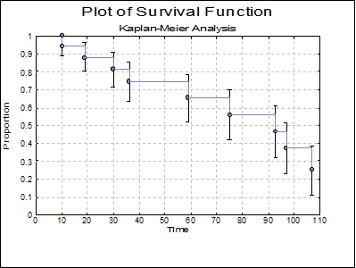
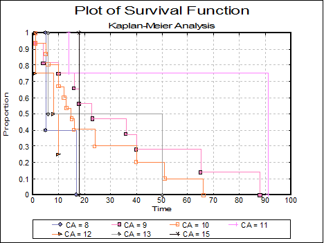
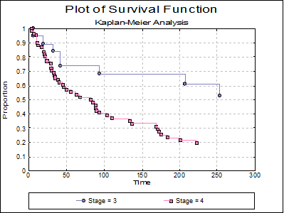
Plot of Survival Function: The cumulative proportion of surviving is plotted against the survival times.

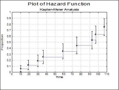
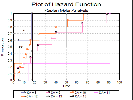
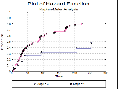
Plot of Hazard Function: The cumulative proportion of terminating is plotted against the survival times.

9.4.2.4. Kaplan-Meier Examples

Example 1

Example 14.1 on p. 479 from Armitage, P. & G. Berry (1994). Data on survival of patients with diffuse hystiocytic lymphoma by the stage of tumour are given.

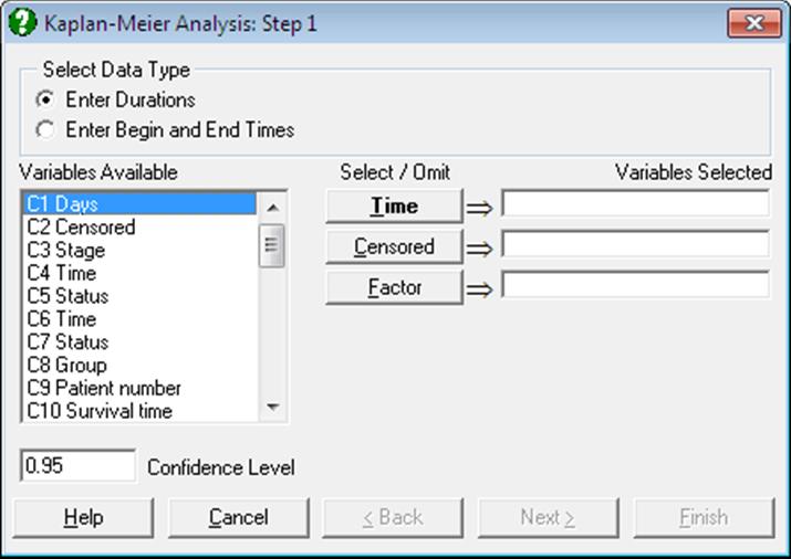
Open SURVIVAL and select Statistics 2 → Survival Analysis → Kaplan-Meier Analysis. From the Variable Selection Dialogue click on the data option 1 Enter Durations and select Days (C1) as [Time], Censored (C2) as [Censored] and Stage (C3) as [Factor]. Select Plot of Survival Function as the output option.

Next click on the [Last Procedure Dialogue] button and this time select Product Limit Survival Table. From the next dialogue check only the Stage = 3 box and then select the first 5 boxes from the Output Options Dialogue to obtain the following output:

Kaplan-Meier Analysis

Product Limit Survival Table

Factor variable: Stage = 3

Time Variable: Days

Censor Variable: Censored

Number of Cases Censored: 11 ( 57.9%)

Valid Number of Cases: 19, 61 Omitted

 

Time	Status	Number Entering	Number Terminating	Cumulative Proportion Surviving	Standard Error of Cumulative Surviving
6	1	18	1	0.9474	0.0512
19	1	17	2	0.8947	0.0704
32	1	16	3	0.8421	0.0837
42	1	15	4	*	*
42	1	14	5	0.7368	0.1010
43	0	13	5	*	*
94	1	12	6	0.6802	0.1080
126	0	11	6	*	*
169	0	10	6	*	*
207	1	9	7	0.6121	0.1167
211	0	8	7	*	*
227	0	7	7	*	*
253	1	6	8	0.5247	0.1287
255	0	5	8	*	*
270	0	4	8	*	*
310	0	3	8	*	*
316	0	2	8	*	*
335	0	1	8	*	*
346	0	0	8	*	*

 

The following graphs are obtained by including stages 3 and 4 in the analysis.

 

 

 

Example 2

Time data in weeks to discontinuation of the use of an IUD is given in Table 1.1 (p. 5), in Collett, D. (1994).

1)       Example 2.3 Table 2.2 (p.21) gives the cumulative survival function.

2)       Example 2.4 Table 2.3 (p.26) gives the cumulative survival function, its standard error and confidence intervals. The 95% confidence intervals reported by Collett are computed by using the standard formula , whereas UNISTAT reports the log-transformed confidence intervals.

3)       Example 2.9 (p.34) gives median and its 95% confidence intervals for cumulative survival function.

Open SURVIVAL and select Statistics 2 → Survival Analysis → Life Table. From the Variable Selection Dialogue select the data option 1 Enter Durations and Survival time (C4) as [Time] and Status (C5) as [Censored].

Kaplan-Meier Analysis

Product Limit Survival Table

Time Variable: time

Censor Variable: status

Number of Cases Censored: 9 ( 50.0%)

Valid Number of Cases: 18, 0 Omitted

 

Time	Status	Number Entering	Number Terminating	Cumulative Proportion Surviving	Standard Error of Cumulative Surviving	Lower 95% of Cumulative Surviving
10	1	17	1	0.9444	0.0540	0.6664
13	0	16	1	*	*	*
18	0	15	1	*	*	*
19	1	14	2	0.8815	0.0790	0.6019
23	0	13	2	*	*	*
30	1	12	3	0.8137	0.0978	0.5241
36	1	11	4	0.7459	0.1107	0.4536
38	0	10	4	*	*	*
54	0	9	4	*	*	*
56	0	8	4	*	*	*
59	1	7	5	0.6526	0.1303	0.3438
75	1	6	6	0.5594	0.1412	0.2564
93	1	5	7	0.4662	0.1452	0.1830
97	1	4	8	0.3729	0.1430	0.1209
104	0	3	8	*	*	*
107	1	2	9	0.2486	0.1392	0.0468
107	0	1	9	*	*	*
107	0	0	9	*	*	*

 

Time	Upper 95% of Cumulative Surviving	Cumulative Proportion Terminating	Standard Error of Cumulative Terminating	Lower 95% of Cumulative Terminating	Upper 95% of Cumulative Terminating
10	0.9920	0.0556	0.0540	0.0080	0.3336
13	*	*	*	*	*
18	*	*	*	*	*
19	0.9691	0.1185	0.0790	0.0309	0.3981
23	*	*	*	*	*
30	0.9363	0.1863	0.0978	0.0637	0.4759
36	0.8970	0.2541	0.1107	0.1030	0.5464
38	*	*	*	*	*
54	*	*	*	*	*
56	*	*	*	*	*
59	0.8432	0.3474	0.1303	0.1568	0.6562
75	0.7804	0.4406	0.1412	0.2196	0.7436
93	0.7097	0.5338	0.1452	0.2903	0.8170
97	0.6310	0.6271	0.1430	0.3690	0.8791
104	*	*	*	*	*
107	0.5313	0.7514	0.1392	0.4687	0.9532
107	*	*	*	*	*
107	*	*	*	*	*

 

Quantiles of Survival Function

Time Variable: time

Censor Variable: status

Number of Cases Censored: 9 ( 50.0%)

Valid Number of Cases: 18, 0 Omitted

Epsilon: 0.05

 

	Value	Standard Error	Lower 95%	Upper 95%
Mean	76.3387	9.4331	57.8502	94.8272
Quantile 1: 25%	107.0000	*	*	*
Quantile 2: 50%	93.0000	17.1311	59.4237	126.5763
Quantile 3: 75%	36.0000	19.9294	*	75.0610