5.3.3. Histogram
Histograms can be drawn with regular or irregular class intervals and with mean, median, mode, lower and upper quartile values displayed. It is possible to fit up to six Distribution Functions simultaneously from a total of 19 continuous and discrete distributions. Frequency distributions and goodness of fit tests are displayed for fitted functions.
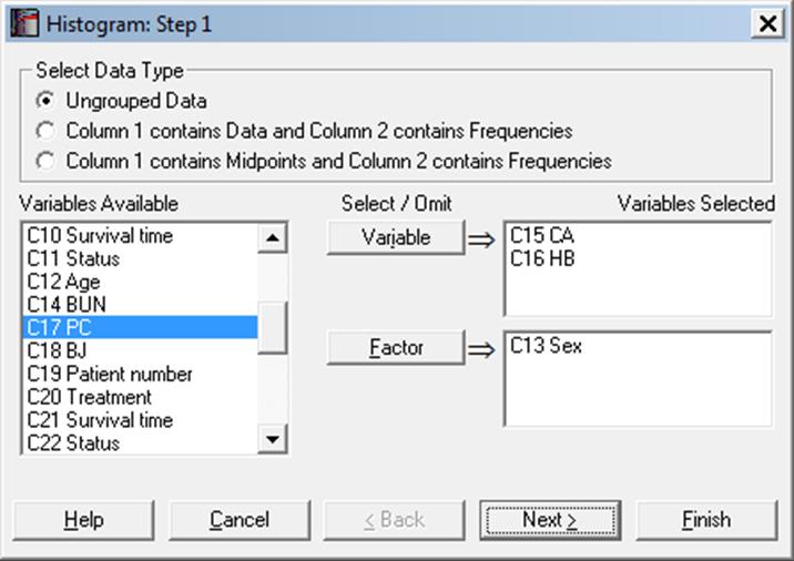
Multisample data can be entered in the form of multiple columns or data columns classified by factor columns. If at least one factor is selected, then a further dialogue will pop up asking for the combination of factor levels to be included. The unchecked levels will be excluded from the plot. If Run a separate analysis for each option selected is checked, a separate output will be generated for each factor level. Otherwise, one histogram will be drawn with the included factor levels.
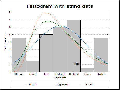
This procedure allows choice of ungrouped data, data with frequency counts or grouped data (see 5.0.2. One-Sample Data Types). It is possible to draw frequency and cumulative histograms for string variables and histograms with irregular class widths.
You can choose to display on the X-axis either the midpoints or the lower and upper limits for each class using the Edit → Bars dialogue.
5.3.3.1. Regular and Irregular Class Intervals
A further dialogue will allow you to edit the number of classes suggested by the program and choose between regular and irregular class intervals. At this stage, the program would already have calculated the default values for the lower and upper bounds and the class interval.
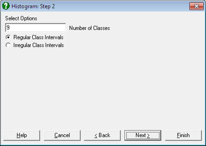
Regular Class Intervals: If this (default) option is selected then the program will proceed with drawing the graph. The lower and upper bound and the class interval values can be edited subsequently, by opening the Edit → Axes dialogue. If the lower limit is higher than the minimum observation or the upper limit is lower than the maximum observation or more than 200 classes are generated, then a warning will be issued. In such cases the program will still proceed with plotting a histogram. If a wider class interval is entered, then the program will not rescale the Y-axis to cater for higher bars. This can be done manually.
For further details of constructing regular class intervals see 5.1.5. Frequency Distributions.
If a string variable is selected, the class intervals will be regular and fixed.
Irregular Class Intervals: If this option is selected then the program will open a new dialogue to allow you to edit the suggested class intervals.
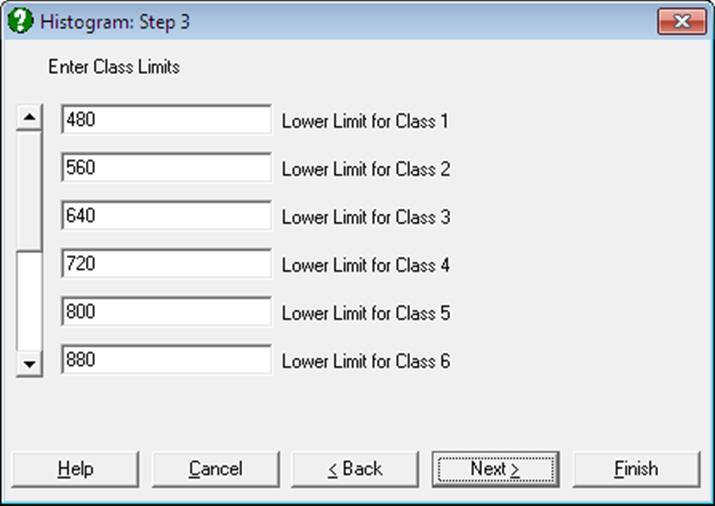
The dialogue contains a vertical scroll bar to edit up to 200 lower limits and the upper limit for the last class. Changes to the number of classes should be made before entering these values. The program will not proceed until a valid selection is made for all classes.
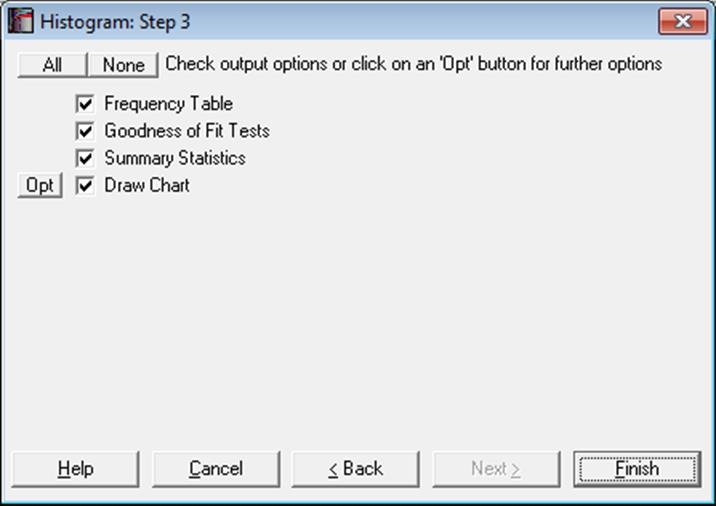
5.3.3.2. Histogram Output Options
The text output from this procedure includes three tables for observed and fitted frequencies, fitted distribution parameters (if any), goodness of fit tests and summary statistics. For the calculation of chi-square statistic and its degrees of freedom see 6.3.1.2. Two Sample Chi-Square Test.
As in other output options (see 2.1.5. Output Options Dialogue), when you click on the [Finish] button, the summary information and the histogram will be sent to the Output Medium with default options. If you want to edit the properties of the histogram, add or remove distribution functions, you can send it to Graphics Editor by clicking on the [Opt] button situated to the left of the Draw Chart check box.
5.3.3.3. Fitting Distribution Functions
When a histogram is displayed with default options, the program will already have fitted eighteen Distribution Functions (except for the negative binomial distribution) on the data. Any six of these can be displayed simultaneously by selecting the Edit → Distributions dialogue. The type, parameters and appearance of these Distribution Functions can be controlled by the user.
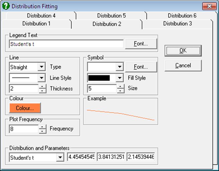
The Edit → Distributions dialogue features a Distribution and Parameters group at the bottom containing a drop-down list for all distributions supported. When a distribution is selected from this list, up to three more text fields are displayed immediately to the right of the list. These fields contain the estimated parameters for each distribution function (see Appendix). For instance, while for the normal distribution two fields will display the estimated mean and standard deviation, for t-distribution a third field will display the estimated degrees of freedom. A parameter which cannot be estimated is assigned the value -99. You can edit the values in each parameter field. For each distribution function you can also select the line style, thickness, colour, symbols, etc.
Any combination of continuous and discrete distribution functions can be selected for up to six distributions. The same distribution can be selected more than once. This may be useful for displaying one or more theoretical curves of the same distribution with different parameters against the fitted parameters.
Distributions in the drop-down list are in the same order as they are in the Distribution Functions dialogue (see 5.2.1. Cumulative Probability). Hypergeometric distribution – for which the estimated frequencies procedure is not implemented – is excluded. It is also possible to plot Distribution Functions without having to fit them on a frequency histogram by means of the Plot of Distribution Functions procedure.
Colour: This controls the colour of the fitted curves.
Symbol: The usual symbol selection group can be used to display Symbols for discrete distributions. When a selection is made other than None for a discrete distribution, a symbol will be drawn on the line at each distinct value of the X-axis variable.
Plot Frequency: This control determines the resolution of fitted distribution curves. The default value of 10 means that the functions will be evaluated at every 10th pixel. This field can have a minimum value of 1, in which case the functions will be evaluated at every pixel. This will take 10 times longer to compute and it may be more difficult to distinguish various curves.
5.3.3.4. Bars
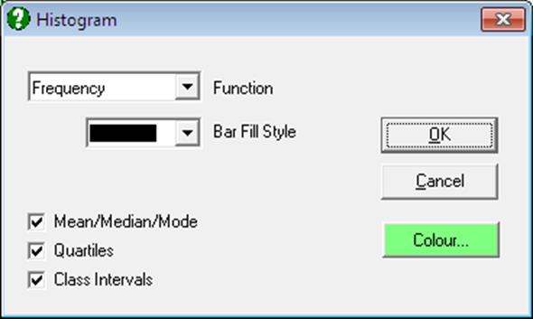
This dialogue provides controls for editing aspects of the histogram bars.
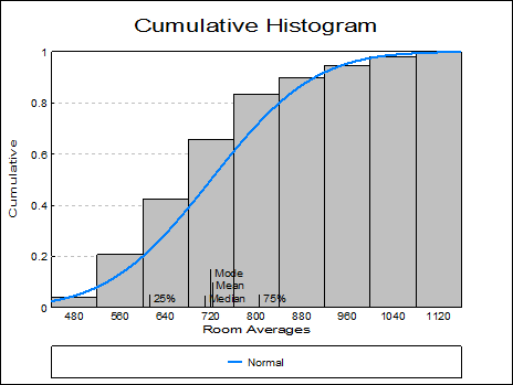
Function: The available options are (i) Frequency and (ii) Cumulative. Distributions can be fitted in either case.
Bar Fill Style: Bars can be filled with solid colours or with cross-hatch patterns.
Bar Colour: This controls the colour of the histogram bars.
Mean / Median / Mode: For numeric variables, this will draw a vertical line for each statistic along the X-axis. For string variables only the mode is drawn.
Quartiles: For numeric variables, a vertical line for 25% and 75% quantiles will be drawn along the X-axis.
Class Intervals: X-axis tick marks and their corresponding value labels can be drawn either in the middle of a class, or at the lower and upper boundaries. This option is available only for histograms with regular class intervals. Irregular histograms will always display class intervals. If the selected column contains String Data, tick marks will always be drawn at midpoints.
5.3.3.5. Example
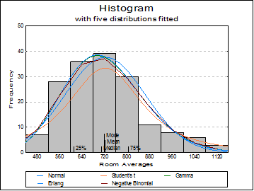
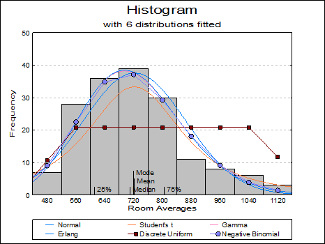
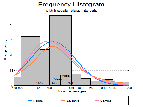
Open TIMESER and select Graph → Descriptive Plots → Histogram. Select Room Averages (C1) as [Variable], accept the program’s suggestion on the next two dialogues and on the Output Options Dialogue, click [Opt] situated to the left of the Draw Chart option. The histogram will be displayed in Graphics Editor. Select Edit → Distributions (or double click at the middle of the graph) and select five distributions as Normal, Student’s t, Gamma, Erlang and Negative Binomial. After the graph is updated, close the Graphics Editor and click [Finish] on the Output Options Dialogue.
Histogram
Frequency Table
|
Room Averages |
Observed |
Normal |
Student’s t |
Gamma |
Erlang |
Negative Binomial |
|
480 |
7.0000 |
9.1004 |
8.8637 |
8.9565 |
8.7975 |
9.0346 |
|
560 |
28.0000 |
19.7499 |
15.9337 |
22.4677 |
22.3912 |
22.5061 |
|
640 |
36.0000 |
31.5472 |
26.3081 |
34.8328 |
34.9867 |
34.8212 |
|
720 |
39.0000 |
37.0937 |
32.6673 |
37.1220 |
37.3794 |
37.1007 |
|
800 |
30.0000 |
32.1072 |
26.8991 |
29.3196 |
29.4695 |
29.2992 |
|
880 |
11.0000 |
20.4574 |
16.4631 |
18.1326 |
18.1278 |
18.1035 |
|
960 |
8.0000 |
9.5939 |
9.1668 |
9.1517 |
9.0733 |
9.1170 |
|
1040 |
6.0000 |
3.3110 |
5.2059 |
3.8914 |
3.8164 |
3.8623 |
|
1120 |
3.0000 |
0.8407 |
3.1213 |
1.4293 |
1.3836 |
1.4110 |
|
Total |
168.0000 |
163.8012 |
144.6289 |
165.3035 |
165.4255 |
165.2557 |
Goodness of Fit
|
|
Parameter 1 |
Parameter 2 |
Parameter 3 |
Chi-Square Statistic |
DoF |
Right-Tail Probability |
|
Normal |
722.2976 |
142.6569 |
|
16.6294 |
6 |
0.0107 |
|
Student’s t |
722.2976 |
142.6569 |
2.0001 |
11.1877 |
5 |
0.0478 |
|
Gamma |
25.6358 |
0.0355 |
|
7.5912 |
6 |
0.2696 |
|
Erlang |
26.0000 |
0.0360 |
|
7.7877 |
6 |
0.2541 |
|
Negative Binomial |
722.2976 |
26.5791 |
|
7.6770 |
6 |
0.2627 |
Descriptive Statistics
|
|
Room Averages |
|
Mean |
722.2976 |
|
Median |
709.5000 |
|
Mode |
720.0000 |
|
Lower Quartile |
612.0000 |
|
Upper Quartile |
805.5000 |