7.3.2. General Linear Model
UNISTAT’s GLM procedure can handle unbalanced designs where the number of observations in cells are not necessarily equal. Data may contain missing values and / or missing cells. Factor columns may be numeric, string, date or time variables and need not be sorted. It is possible to select an unlimited number of dependent variables, factors, repeated measures and covariates. When more than one dependent variable is selected, the analysis will be repeated for each dependent variable with the rest of the settings unchanged.
The GLM procedure assumes that each factor has a maximum of 1000 levels, though this number may be increased by the user, if necessary. It is possible to analyse simple factorial, repeated measures, nested and mixed designs. The output options include table of means, coefficients, fitted values and residuals and their plots. It is also possible to perform multiple comparison tests on the GLM model fitted.
This procedure allows more flexibility in defining the ANOVA model to be used. All the previous models can be built using the General Linear Model procedure. Also, this procedure can handle 4 way and above interactions / nested terms and allows the specification of the F-ratio terms.
The GLM procedure always adopts the Regression Approach to sum of squares. This means the factors can be selected in any order and the same sum of squares will be obtained.
7.3.2.1. GLM Variable Selection
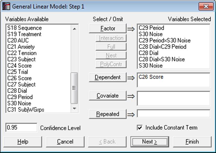
The variable selection for General Linear Model is slightly different from the ANOVA procedures. When a selection is made from the Variables Available list on the left, the variable remains there, allowing it to be selected again. The [Dependent] and [Covariate] buttons work as before (see 7.3.1.1. ANOVA Variable Selection). The [Factor], [Interaction], [Full] and [Nest] all add factors to the factor list box. They do this in the following way:
Factor: is used to select a single factor variable. If multiple variables are highlighted in the Variables Available list, then all these variables will be added to the factors list.
Interaction: is used to select an interaction term. This will only be active when multiple variables are selected in the Variables Available list. A single factor of the form FactA x FactB x … is added. You can always highlight multiple nonadjacent variables by pressing on the [Ctrl] key and then clicking on the desired variable.
A special cross sign is used between the variables in an interaction term. If there is a problem with this character on a non-English operating system, you can enter and edit the following line in Documents\Unistat10\Unistat10.ini file under [Options] to display any other character (say x):
InteractionCross=x
This character also appears in all ANOVA and GLM output with interaction terms.
Full: is used to add all the factors and interactions for a fully factorial model. This will only be active when multiple variables are selected in the Variables Available list. You can always highlight multiple nonadjacent variables by pressing on the [Ctrl] key and then clicking on the desired variable.
Nest: is used to create a nested term. This will only be active when a variable is selected in the Variables Available list and a factor is highlighted in the factors list on the right. When selected, this will create a nested factor of the form FactA(FactB). This can be repeated to create a multilevel nested factor e.g. FactA(FactB(FactC)). Nests on interactions, such as FactA(FactB x FactC), are not allowed.
PolyContr: This button is used to request orthogonal polynomial contrasts for factors or interactions of factors. When a factor or interaction term is selected on the Variables Selected list, the [PolyContr] button will be enabled. The selected factors should contain minimum two and maximum six levels. Otherwise the polynomial contrasts cannot be computed. Contrasts for interaction terms are obtained from the dummy variables created for the main factors.
Polynomial contrasts should be used when the factor levels are equally spaced, although UNISTAT will not check for this condition and compute contrasts anyway.
The following table shows the coefficients used in dummy variables for factors with two to six levels. Each coefficient is divided by the Divisor displayed on the right of the table.
|
Factor Levels |
Polynomial Degree |
D1 |
D2 |
D3 |
D4 |
D5 |
D6 |
Divisor |
|
2 |
1 |
-1 |
1 |
2 |
||||
|
3 |
1 |
-1 |
0 |
1 |
2 |
|||
|
2 |
1 |
-2 |
1 |
6 |
||||
|
4 |
1 |
-3 |
-1 |
1 |
3 |
20 |
||
|
2 |
1 |
-1 |
-1 |
1 |
4 |
|||
|
3 |
-1 |
3 |
-3 |
1 |
20 |
|||
|
5 |
1 |
-2 |
-1 |
0 |
1 |
2 |
10 |
|
|
2 |
2 |
-1 |
-2 |
-1 |
2 |
14 |
||
|
3 |
-1 |
2 |
0 |
-2 |
1 |
10 |
||
|
4 |
1 |
-4 |
6 |
-4 |
1 |
70 |
||
|
6 |
1 |
-5 |
-3 |
-1 |
1 |
3 |
5 |
70 |
|
2 |
5 |
-1 |
-4 |
-4 |
-1 |
5 |
84 |
|
|
3 |
-5 |
7 |
4 |
-4 |
-7 |
5 |
180 |
|
|
4 |
1 |
-3 |
2 |
2 |
-3 |
1 |
28 |
|
|
5 |
-1 |
5 |
-10 |
10 |
-5 |
1 |
252 |
Dependent: It is compulsory to select at least one column containing numeric data. When more than one data variable is selected, the analysis will be repeated as many times as the number of data variables, each time only changing the data variable and keeping the rest of selections unchanged.
Covariate: A covariate is a continuous (noncategorical) numeric variable that may be included in the analysis in order to remove its effect on the dependent variable. Any number of covariates can be selected from the Variables Available list by clicking on [Covariate]. When covariates are included in the analysis, an adjustment is made in the sum of squares for them before any other factors.
Repeated: This button is used to select a factor to define Within and Between Subjects terms. These can be used in the F-ratio selection to create a number of different repeated measure designs. If a variable is selected as [Repeated], then at least one factor must use the Error Within term in its F-ratio (see 7.3.2.2. GLM F-Ratio Selection).
7.3.2.2. GLM F-Ratio Selection
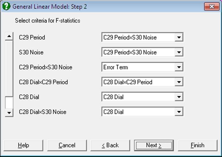
This dialogue allows the denominator in the F-ratio of each factor to be specified independently. The possible selections include:
Residual: The denominator is given by the total error of the model. This is the default in GLM and it is also the denominator used in ANOVA.
None: The F-statistic and its tail probability are not calculated.
Error Term: The factor is not included in the model – also known as Fixed Factor. That is, the sum of squares calculated is not included in the explained sum of squares and hence the residual sum of squares is not adjusted for this factor. The sum of squares is reported separately from the factors included in the model. R-squared and adjusted R-squared are not reported for a model that includes error terms.
Any Factor’s Mean Square: The denominator is given by the mean square of the selected factor.
Error Between Subjects: This option will only be available when a column is selected as [Repeated] in the variable selection. The denominator is given by the Error Between Subjects mean square. This value is calculated by the sum of squares of the selected column minus the sum of square of all the factors with denominator selected as Error Between Subjects. So the mean square value depends on which factors are selected as Error Between Subjects.
Error Within Subjects: This option will only be available when a column is selected as [Repeated] in the variable selection. This term partitions the residual sum of squares with the Error Between Subjects. So the mean square value depends on which factors are selected as Error Between Subjects.
7.3.2.3. GLM Output Options
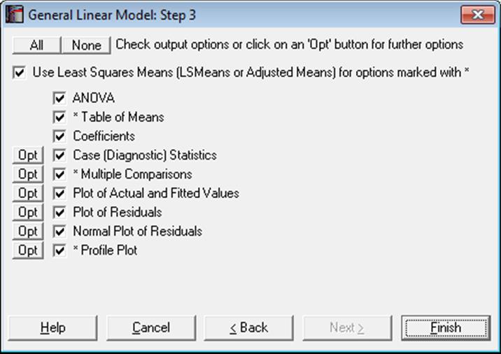
The main output of the GLM procedure is the ANOVA table. However, GLM also reports a wide range of diagnostic statistics, post hoc tests and plots.
As of this version of UNISTAT, three more options have been added to the Output Options Dialogue. It is now possible to include any or all three output tables for each test.
Use Least Squares Means: The following three output options are preceded by an asterisk in the Output Options Dialogue;
· Table of Means,
· Multiple Comparisons and
· Profile Plot.
The common point for these options is that they display information based on cell and / or marginal means (where a cell is defined as a unique combination of factor levels used in the model and a marginal mean is the mean of a group of cell means). It is possible to display these output options based on the least squares means (LSMeans or adjusted means) instead of arithmetic means. To do this check the Use Least Squares Means box at the top of the dialogue. Then these three output options will use the least squares means and this will be indicated on the output. Note that the least squares means output will not be available when a nested term exists in the model.
Normally, in balanced designs arithmetic and least squares means will not be different. However, in unbalanced designs with more than one effect, the arithmetic mean of a group may not represent an appropriate response for that group, since it does not take other effects in the model into account. Least squares means can also be described as within-group means adjusted for the other effects in the model. In other words, least squares means are predicted population margins which estimate the marginal means over a balanced population.
The least squares means are computed as:
![]()
where L is the hypothesis matrix and ![]() is the vector of estimated regression
coefficients as displayed in the third output option:
is the vector of estimated regression
coefficients as displayed in the third output option:
![]()
The standard error of LSMeans is defined as:
![]()
where MSE is the mean square error for the model.
To save the hypothesis matrix L in a file enter the following line under the [Options] section of Documents\Unistat10\Unistat10.ini file:
GLMSaveLMatrix=1
The matrix will be saved in:
..\Documents\Unistat10\GLMLMatrix.txt
To save the ![]() matrix enter the following line under
the [Options] section of Unistat10.ini:
matrix enter the following line under
the [Options] section of Unistat10.ini:
GLMSaveInvXpXMatrix=1
The matrix will be saved in the file:
..\Documents\Unistat10\GLMInvXpXMatrix.txt
Some of the GLM Output Options (such as coefficients, fitted values, residuals and their plots) are based on the underlying regression model for the GLM model. These are normally identical to the results obtained from the Linear Regression procedure if the same model is constructed using dummy variables (see 7.3.2.4. GLM Example below).
ANOVA: The factors in the model appear at the top of the table. Any factors that have been calculated but are not in the model appear at the bottom of the table in a section separated with a dividing line. These values may be used as denominators in F-statistic calculations. If a repeated measure has been specified, then the factor will be split into Between Subjects and Within Subjects terms.
* Table of Means: Number of cases, mean, standard deviation, standard error and the lower and upper limits of the confidence interval are displayed for each cell and marginal mean of the model. Missing cells are omitted from the analysis at the outset. This output option is similar to the Table of Means procedure available under Tests for ANOVA, but has the advantage of matching exactly the model specified in the GLM procedure. When the Use Least Squares Means box is checked, LSMeans will be displayed instead of arithmetic means.
Coefficients: Estimated coefficients for the underlying regression model are displayed. The Row Labels of this table are identical to that of Table of Means output above. Variables causing multicollinearity will be displayed with a zero coefficient at the end of the coefficients table. If you do not wish to display these variables enter the following line in the [Options] section of Documents\Unistat10\Unistat10.ini file:
DispCollin=0
Case (Diagnostic) Statistics: The actual, fitted and residual Y values for the underlying regression model are displayed.
* Multiple Comparisons: This output option is similar to the Multiple Comparisons procedure available under Tests for ANOVA, but has a major advantage. While the latter is always based on a one-way ANOVA model, this option takes the Mean Square Error and its Degrees of Freedom from the estimated GLM model. Note that both procedures give you the opportunity to override the suggested Mean Square Error and its Degrees of Freedom. When the Use Least Squares Means box is checked, comparisons will be made between LSMeans instead of arithmetic means.
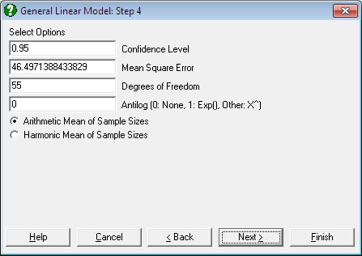
When the data used in multiple comparisons is already transformed with a function like e or 10 based logarithm, the results need to be transformed back to the original scale and the user is faced with the task of applying back transformations manually. The Antilog box allows the user to specify which back-transformation is to be applied in the output. The output values that are affected by this control are:
· means,
· difference between means, and
· lower and upper confidence limits for difference between means.
Let X be the value entered into the Antilog box.
· If X = 0 then no back-transformation is performed.
· If X = 1 then the natural antilog of the output value Y, Exp(Y) is displayed.
· If 1 < X ≤ 16, then X-based power of Y, X^Y is displayed.
When a back-transformation base value is specified, the columns affected will be marked by an asterisk in the output.
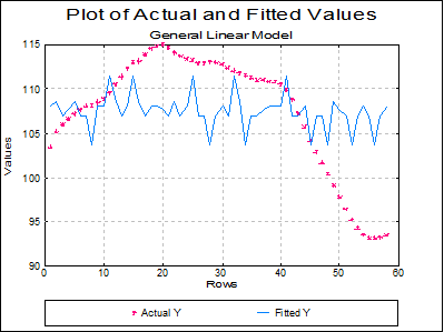
Plot of Actual and Fitted Values: Select this option to plot actual and fitted Y values against row numbers (index).
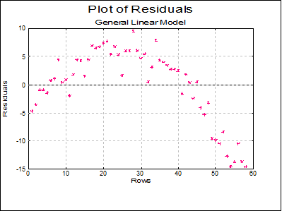
Plot of Residuals: Residuals are plotted against row numbers (index).
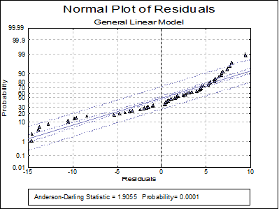
Normal Plot of Residuals: Residuals are plotted against the normal probability (probit) axis.
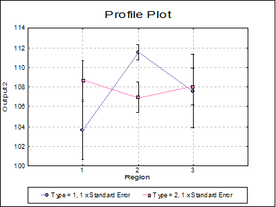
* Profile Plot: The cell means for an unlimited number of factors can be plotted. If only one factor is selected, the plot is similar to the Means Plot with Error Bars option available in X-Y Plots (see 4.1.1.3. Means Plot). When the Use Least Squares Means box is checked, LSMeans will be plotted instead of arithmetic means.
If two or more factors are selected, the first factor’s levels are represented on the X-Axis and the second factor’s levels as separate lines. This plot is known as Interaction Plot and it is different from a Means Plot with two factors (where interaction terms are plotted either on the X-Axis or as separate lines). The Interaction Plot is useful for comparing means of interaction terms. If the lines are parallel, then it can be concluded that there is no interaction between the two factors.
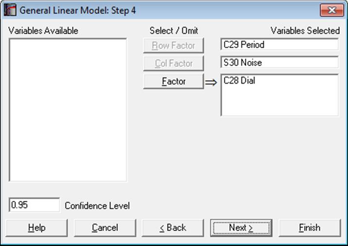
To change the default factor selections, you can click on the [Opt] button situated to the left of this output option. A further Variable Selection Dialogue is displayed. It is compulsory to select a [Row Factor] variable, in which case a Means Plot is displayed for the selected factor. If an optional [Column Factor] is also selected, then an Interaction Plot is displayed.
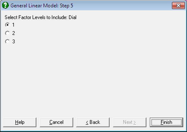
A third [Factor] button allows selection of an unlimited number of further factor columns. If at least one such factor is selected, then the program displays a further dialogue showing the levels of this factor. If two or more factors are selected then the dialogue shows the combinations of all selected factors. Only one level (or level combination) needs to be selected and the final plot is drawn for this selected subsample. When [Factor] columns are selected, selection of a [Column Factor] still remains optional.
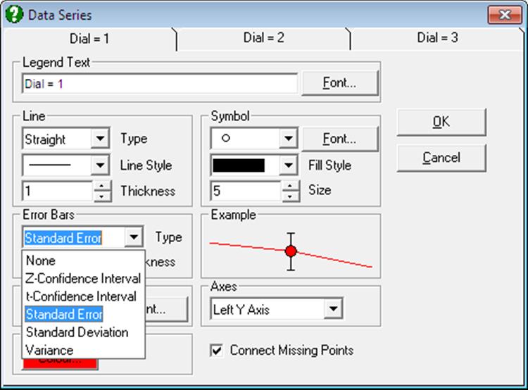
In earlier versions of UNISTAT, error bars for means plot represented only the standard error of mean. Now, (as in Means Plot), the Error Bars control on the Edit → Data Series dialogue allows selecting one of the following dispersion measures: None, t-interval, Z-interval, Standard Error, Standard Deviation, Variance
7.3.2.4. GLM Example
Published examples using GLM have already been introduced in section 7.3.0.2. ANOVA Designs. Here we shall demonstrate the full GLM output with a simple example. Next, we shall run the same model using the Linear Regression procedure and emphasise the similarities and differences.
Open DEMODATA and select Statistics 1 → ANOVA and GLM → General Linear Model. Highlight Region (C10) and Type (C11) on the Variables Available list and then click on the button [Full]. This will add two main factors and an interaction term to the Variables Selected list. Also select Output2 (C9) as [Dependent]. Accept default values suggested in the next two dialogues. Some of the following results have been shortened due to space considerations.
General Linear Model
ANOVA
Dependent Variable: Output2
|
Due To |
Sum of Squares |
DoF |
Mean Square |
F-Stat |
Prob |
|
Constant |
669862.660 |
1 |
669862.660 |
281.165 |
0.0000 |
|
Region |
70.934 |
2 |
35.467 |
0.774 |
0.4664 |
|
Type |
1.122 |
1 |
1.122 |
0.024 |
0.8762 |
|
Region x Type |
174.832 |
2 |
87.416 |
1.908 |
0.1586 |
|
Explained |
206.738 |
5 |
41.348 |
0.902 |
0.4866 |
|
Error |
2382.454 |
52 |
45.816 |
|
|
|
Total |
2589.193 |
57 |
45.424 |
|
|
|
R-squared = |
0.0798 |
|
Adjusted R-squared = |
-0.0086 |
Table of Means
|
|
Cases |
Mean |
Standard Deviation |
Standard Error |
Lower 95% |
Upper 95% |
|
whole sample |
58 |
107.4679 |
6.7398 |
0.8850 |
105.6958 |
109.2401 |
|
Region = 1 |
14 |
106.1586 |
6.9131 |
1.8476 |
102.1671 |
110.1501 |
|
2 |
26 |
107.8269 |
6.7597 |
1.3257 |
105.0966 |
110.5572 |
|
3 |
18 |
107.9678 |
6.8330 |
1.6106 |
104.5698 |
111.3658 |
|
Type = 1 |
16 |
107.0837 |
6.9366 |
1.7342 |
103.3875 |
110.7800 |
|
2 |
42 |
107.6143 |
6.7430 |
1.0405 |
105.5130 |
109.7156 |
|
Region x Type = 1 x 1 |
7 |
103.6271 |
7.7791 |
2.9402 |
96.4327 |
110.8216 |
|
1 x 2 |
7 |
108.6900 |
5.2991 |
2.0029 |
103.7892 |
113.5908 |
|
2 x 1 |
5 |
111.5200 |
1.7219 |
0.7701 |
109.3820 |
113.6580 |
|
2 x 2 |
21 |
106.9476 |
7.2320 |
1.5782 |
103.6557 |
110.2396 |
|
3 x 1 |
4 |
107.5875 |
7.3881 |
3.6940 |
95.8315 |
119.3435 |
|
3 x 2 |
14 |
108.0764 |
6.9572 |
1.8594 |
104.0594 |
112.0934 |
Coefficients
|
|
Coefficient |
Standard Error |
t-Statistic |
Probability |
Lower 95% |
Upper 95% |
|
Constant |
108.0764 |
1.8090 |
59.7426 |
0.0000 |
104.4463 |
111.7065 |
|
Region = 1 |
0.6136 |
3.1333 |
0.1958 |
0.8455 |
-5.6740 |
6.9011 |
|
2 |
-1.1288 |
2.3355 |
-0.4833 |
0.6309 |
-5.8153 |
3.5576 |
|
3 |
* |
|
|
|
|
|
|
Type = 1 |
-0.4889 |
3.8375 |
-0.1274 |
0.8991 |
-8.1895 |
7.2117 |
|
2 |
* |
|
|
|
|
|
|
Region x Type = 1 x 1 |
-4.5739 |
5.2742 |
-0.8672 |
0.3898 |
-15.1574 |
6.0096 |
|
1 x 2 |
* |
|
|
|
|
|
|
2 x 1 |
5.0613 |
5.1060 |
0.9912 |
0.3262 |
-5.1848 |
15.3074 |
|
2 x 2 |
* |
|
|
|
|
|
|
3 x 1 |
* |
|
|
|
|
|
|
3 x 2 |
* |
|
|
|
|
|
* omitted due to multicollinearity
Case (Diagnostic) Statistics
|
|
Actual Y |
Fitted Y |
Residuals |
|
1 |
103.3600 |
108.0764 |
-4.7164 |
|
2 |
105.1300 |
108.6900 |
-3.5600 |
|
3 |
105.9700 |
106.9476 |
-0.9776 |
|
… |
… |
… |
… |
|
56 |
93.1100 |
103.6271 |
-10.5171 |
|
57 |
93.2000 |
106.9476 |
-13.7476 |
|
58 |
93.4700 |
108.0764 |
-14.6064 |
Dunnett
For Output2, classified by Region
Control Group: 1, Two-Tailed Test
Mean Square Error: 45.8164292353523, Degrees of Freedom: 52
** denotes significantly different pairs. Vertical bars show homogeneous subsets.
A pairwise test result is significant if its q stat value is greater than the table q.
|
Group |
Cases |
Mean |
1 |
|
|
1 |
14 |
106.1586 |
|
| |
|
2 |
26 |
107.8269 |
|
| |
|
3 |
18 |
107.9678 |
|
| |
|
Comparison |
Difference |
Standard Error |
q Stat |
Table q |
Probability |
|
3 – 1 |
1.8092 |
2.4120 |
0.7501 |
2.2581 |
0.6578 |
|
2 – 1 |
1.6684 |
2.2438 |
0.7435 |
2.2581 |
0.6623 |
|
Comparison |
Lower 95% |
Upper 95% |
Result |
|
3 – 1 |
-3.6375 |
7.2559 |
|
|
2 – 1 |
-3.3985 |
6.7352 |
|
|
Homogeneous Subsets: |
|
|
Group 1: |
1 2 3 |
|
Pooled mean = |
107.4679 |
|
95% Confidence Interval = |
105.6845 <> 109.2514 |
Now we run the same model using Linear Regression.
Open DEMODATA and select Statistics 1 → Regression Analysis → Linear Regression. Highlight Region (C10) and Type (C11) on the Variables Available list and then click on the button [Full]. This will add two main factors and an interaction term to the Variables Selected list. Also select Output2 (C9) as [Dependent]. From the Output Options Dialogue select only the Regression Results and ANOVA of Regression. The following results are obtained.
The Regression Results option produces exactly the same results as the GLM model. In the ANOVA of Regression table, Regression, Error and Total terms are also identical to Explained, Error and Total of GLM’s ANOVA table. Moreover, if we add the two interaction Ssq’s (1×1 and 2×1) we obtain the Region x Type Ssq of GLM. Main interactions are, however, different. This is because the GLM Procedure adopts the Regression Approach when it computes the sum of squares, whereas Linear Regression’s sum of squares decomposition is sequential. See 7.3.1.3. ANOVA Approaches.
Linear Regression
Dependent Variable: Output2
Valid Number of Cases: 58, 0 Omitted
Regression Results
* omitted due to multicollinearity
|
|
Coefficient |
Standard Error |
t-Statistic |
Probability |
Lower 95% |
Upper 95% |
|
Constant |
108.0764 |
1.8090 |
59.7426 |
0.0000 |
104.4463 |
111.7065 |
|
Region = 1 |
0.6136 |
3.1333 |
0.1958 |
0.8455 |
-5.6740 |
6.9011 |
|
2 |
-1.1288 |
2.3355 |
-0.4833 |
0.6309 |
-5.8153 |
3.5576 |
|
Type = 1 |
-0.4889 |
3.8375 |
-0.1274 |
0.8991 |
-8.1895 |
7.2117 |
|
Region x Type = 1 x 1 |
-4.5739 |
5.2742 |
-0.8672 |
0.3898 |
-15.1574 |
6.0096 |
|
2 x 1 |
5.0613 |
5.1060 |
0.9912 |
0.3262 |
-5.1848 |
15.3074 |
|
Region = 3 |
* |
|
|
|
|
|
|
Type = 2 |
* |
|
|
|
|
|
|
Region x Type = 1 x 2 |
* |
|
|
|
|
|
|
2 x 2 |
* |
|
|
|
|
|
|
3 x 1 |
* |
|
|
|
|
|
|
3 x 2 |
* |
|
|
|
|
|
|
Residual Sum of Squares = |
2382.4543 |
|
Standard Error = |
6.7688 |
|
Mean of Y = |
107.4679 |
|
Stand Dev of y = |
6.7398 |
|
Correlation Coefficient = |
0.2826 |
|
R-squared = |
0.0798 |
|
Adjusted R-squared = |
-0.0086 |
|
F(5,52) = |
0.9025 |
|
Probability of F = |
0.4866 |
|
Durbin-Watson Statistic = |
0.1641 |
|
log of likelihood = |
-190.2131 |
|
Press Statistic = |
2916.1898 |
ANOVA of Regression
|
Due To |
Sum of Squares |
DoF |
Mean Square |
F-Stat |
Prob |
|
Region = 1 |
31.639 |
1 |
31.639 |
0.691 |
0.4098 |
|
2 |
0.211 |
1 |
0.211 |
0.005 |
0.9462 |
|
Type = 1 |
0.057 |
1 |
0.057 |
0.001 |
0.9721 |
|
Region x Type = 1 x 1 |
129.815 |
1 |
129.815 |
2.833 |
0.0983 |
|
2 x 1 |
45.017 |
1 |
45.017 |
0.983 |
0.3262 |
|
Regression |
206.738 |
5 |
41.348 |
0.902 |
0.4866 |
|
Error |
2382.454 |
52 |
45.816 |
|
|
|
Total |
2589.193 |
57 |
45.424 |
0.991 |
0.5142 |