7.4.3. Multiple Comparisons
Multiple comparisons (also known as multiple range, post hoc or a posteriori tests) are designed to compare all possible pairs of means of a group of subsamples. These tests are usually performed after an ANOVA, where the null hypothesis “all population means are equal” is rejected. The null hypotheses “mean A is equal to mean B”, “mean A is equal to mean C”, etc. can be tested for all k(k – 1)/2 pairs of k subgroups. It is also possible to test all subgroups against a control subgroup (Dunnett test), in which case only k – 1 comparisons are made.
Comparisons are performed on subgroups of a single factor column, corresponding to a one-way analysis. However, the user can perform comparisons based on any ANOVA model by entering the Mean Square Error (MSE) and its Degrees of Freedom manually.
All tests are of the following general form:
![]()
where q(α,k,f) is the range at α significance level, k is the number of subsets, f is the degrees of freedom of the between-groups sum of squares and Sx is the combined standard error. The combined standard error can be weighted by an arithmetic (the default) or harmonic mean of sample sizes. Although the latter is generally used when the sample sizes are not all equal, in such cases UNISTAT will not automatically revert to the harmonic mean. The selection should be made by the user, if the harmonic mean is required.
By default, the test result is reported by comparing a pair’s observed q value against the table q for the given significance level and degrees of freedom. However, if required, comparisons can be made according to the probability value or confidence interval. To select one of these options, the following line should be entered and edited in the [Options] section of Documents\Unistat10\ Unistat10.ini file:
ComparisonCriterion=i
where:
· i = 1: Critical value: Significant when the observed q value is greater than the table q (except for the upper-tailed Dunnett test).
· i = 2: Probability: Significant when the observed p-value is less than the given significance level (0.05 is the default).
· i = 3: Confidence interval: Significant when the confidence interval does not include zero.
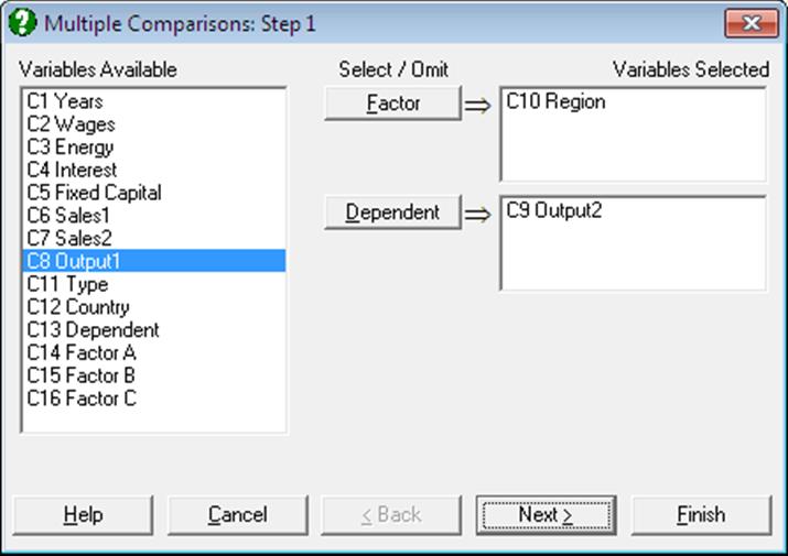
Select at least one data column by clicking on [Dependent] and at least one factor column by clicking on [Factor], which separates the data column into a number of subgroups (or treatments). The procedure is run separately for each [Factor] / [Dependent] pair. A one-way ANOVA model is estimated and the Mean Square Error and its Degrees of Freedom are displayed in a dialogue.
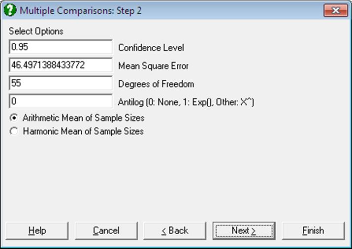
The ability to edit these values enables the user to make comparisons based on any ANOVA model. For instance, if you wish to perform Multiple Comparisons for a 3-way ANOVA, you can copy the Mean Square Error and its Degrees of Freedom from the 3-way ANOVA table and paste them into the respective text boxes on this dialogue. Here you can also change the significance level and choose between arithmetic and harmonic means for sample sizes.
Back Transformations: Often, the data used in Multiple Comparisons is already transformed with a function like e or 10 based logarithm. In such cases the results need to be transformed back to the original scale and the user is faced with the task of applying back transformations manually. The Antilog box allows the user to specify which back-transformation is to be applied in the output. The output values that are affected by this control are:
· means,
· difference between means, and
· lower and upper confidence limits for difference between means.
Let X be the value entered into the Antilog box.
· If X = 0 then no back-transformation is performed.
· If X = 1 then the natural antilog of the output value Y, Exp(Y) is displayed.
· If 1 < X ≤ 16, then X based power of Y, X^Y is displayed.
When a back-transformation base value is specified, the columns affected will be marked by an asterisk in the output.
Next the Output Options Dialogue is displayed. As of this version of UNISTAT, this dialogue features three new check boxes for the three main components of Multiple Comparisons output; Comparison Table, Pairwise Tests and Homogeneous Subsets.
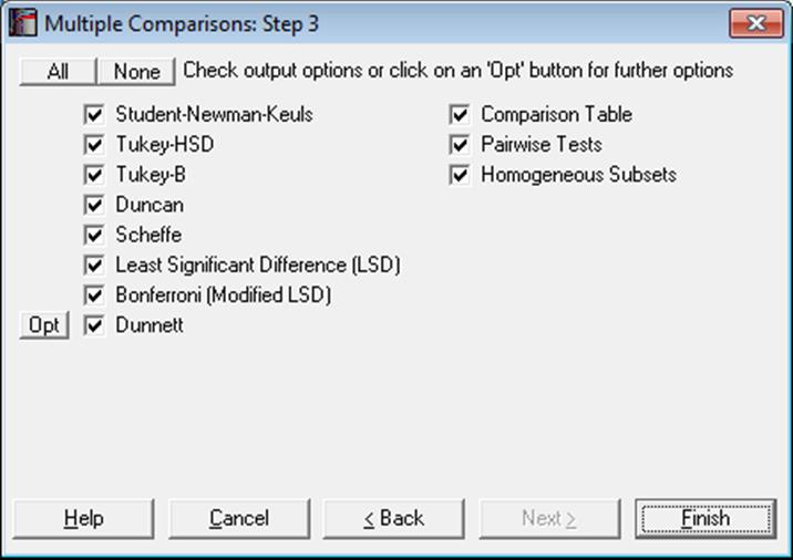
Some or all of the eight comparison tests can be selected for output.
2) Tukey-HSD
3) Tukey-B
4) Duncan
5) Scheffe
6) Least Significant Difference (LSD)
8) Dunnett
The Dunnett test is different from the others in that it requires selection of a control group and allows selection of two-tailed, lower and upper tail tests. These dialogues are accessible from the [Opt] button situated immediately to the left of the Dunnett check box. By default, the control group is the first group of sorted factor levels and a two-tailed test is performed.
These tests are covered in standard textbooks for experimental design (e.g. Montgomery, D. C. (1991). The present implementation is based on Winer, B. J. (1970).
Multiple Comparisons are also available following a GLM analysis, where the Mean Square Error is based on the error term of the model fitted and therefore there is no need to copy and paste any values (see 7.3.2. General Linear Model).
Comparison Table: The output includes a comparison matrix where significantly different pairs are marked with an asterisk. Where appropriate, the groups are divided into homogenous subsets where their differences are not significant according to the given significance criterion. Vertical bars on the right of the table indicate the homogeneous subsets. Homogeneous subsets are not available for all tests.
Pairwise Tests: A second table displays the pairs compared, their difference, standard error, observed and table q statistics, probability, confidence interval and the test result. Double asterisks are displayed on the last column, if the difference between two means is significantly different from zero. By design, confidence intervals are not available for Student-Newman-Keuls and Duncan methods.
Homogeneous Subsets: The third part of output will list homogenous subsets, their pooled mean and confidence intervals. The critical values are based on t-distribution. Differences between pooled means of homogenous subsets and their confidence intervals are also displayed. Critical values are based on the studentised t-distribution.
Another way to shorten the Multiple Comparisons output is to enter the following line in the [Options] section of Documents\Unistat10\Unistat10.ini file:
ComparisonShortOutput=1
In this case, only a comparison table will be displayed, the contents of which depend on the comparison criterion selected by the ComparisonCriterion entry as described above. If ComparisonCriterion=2, then the short output will display only the observed probability and the test result based on probability. If ComparisonCriterion=3, then the short output will display only the confidence interval and the test result based on whether it contains zero.
UNISTAT also offers a number of nonparametric Multiple Comparisons, comparisons of medians, variances and intercepts and slopes of regression lines. The full list of these procedures and the available Multiple Comparisons is as follows:
Statistics 1 → Nonparametric Tests (Multisample) → Kruskal-Wallis ANOVA
Nonparametric comparisons against a control group:
Dunnett, Dunn.
Nonparametric comparisons:
with rank sums: Tukey, S-N-K
with mean ranks: Tukey, S-N-K
t, Dunn
Statistics 1 → Nonparametric Tests (Multisample) → Multisample Median Test
Multiple comparison of medians: Tukey
Statistics 1 → Nonparametric Tests (Multisample) → Friedman Two-Way ANOVA
Nonparametric Multiple Comparisons: Tukey
Statistics 1 → Nonparametric Tests (Multisample) → Quade Two-Way ANOVA
Nonparametric Multiple Comparisons: Tukey
Statistics 1 → Tests for ANOVA → Homogeneity of Variance Tests
Comparison of variances against a control group: Dunnett
Multiple comparison of variances: Tukey, S-N-K
Statistics 1 → Tests for ANOVA → Heterogeneity of Regression
Comparison of slopes against a control group: Dunnett
Comparison of intercepts against a control group: Dunnett
Multiple comparison of slopes: Tukey
Multiple comparison of intercepts: Tukey
By default, these procedures will display all three main components of the multiple comparisons output; Comparison Table, Pairwise Tests and Homogeneous Subsets. If you wish to make the output from them to obey the Multiple Comparisons Output Options Dialogue check boxes, to display only the selected parts of the output, enter the following line in the [Options] section of Documents\Unistat10\Unistat10.ini file:
MultiCompOthers=1
7.4.3.1. Student-Newman-Keuls
Student-Newman-Keuls procedure is based on the studentised range and has different range values for different size subsets. Comparisons can be made at any confidence level.
The standard error is defined as:
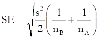
Confidence intervals are not available for this test due to its multistage character.
Example
Examples 11.1 and 11.4 on p. 228 and p. 234 from Zar, J. H. (2010). A researcher wants to find out which variables have different means at a 95% confidence level.
The table format given in the book can be transformed into the factor format by using UNISTAT’s Data → Stack Columns procedure and the Level() function (see 3.4.2.5. Statistical Functions). All data should be stacked in a single column Concentration and a factor column Water created to keep track of the group memberships.
Open ANOTESTS, select Statistics 1 → Tests for ANOVA → Multiple Comparisons, Water (C3) as [Factor] and Concentration (C4) as [Dependent], click [Next] to accept default values at the next dialogue and select Student-Newman-Keuls to obtain the following results:
Multiple Comparisons
Student-Newman-Keuls
For Concentration, classified by Water
Mean Square Error: 9.7652, Degrees of Freedom: 25
** denotes significantly different pairs. Vertical bars show homogeneous subsets.
A pairwise test result is significant if its q stat value is greater than the table q.
|
Group |
Cases |
Mean |
1 |
2 |
4 |
3 |
5 |
|
|
1 |
6 |
32.0833 |
|
** |
** |
** |
** |
| |
|
2 |
6 |
40.2333 |
** |
|
|
|
** |
| |
|
4 |
6 |
41.1000 |
** |
|
|
|
** |
| |
|
3 |
6 |
44.0833 |
** |
|
|
|
** |
| |
|
5 |
6 |
58.3000 |
** |
** |
** |
** |
|
| |
|
Comparison |
Difference |
Standard Error |
q Stat |
Table q |
Probability |
|
5 – 1 |
26.2167 |
1.8042 |
20.5500 |
4.1534 |
0.0000 |
|
3 – 1 |
12.0000 |
1.8042 |
9.4062 |
3.8900 |
0.0000 |
|
4 – 1 |
9.0167 |
1.8042 |
7.0677 |
3.5226 |
0.0001 |
|
2 – 1 |
8.1500 |
1.8042 |
6.3884 |
2.9126 |
0.0001 |
|
5 – 2 |
18.0667 |
1.8042 |
14.1616 |
3.8900 |
0.0000 |
|
3 – 2 |
3.8500 |
1.8042 |
3.0178 |
3.5226 |
0.1032 |
|
4 – 2 |
0.8667 |
1.8042 |
0.6793 |
2.9126 |
0.6351 |
|
5 – 4 |
17.2000 |
1.8042 |
13.4823 |
3.5226 |
0.0000 |
|
3 – 4 |
2.9833 |
1.8042 |
2.3385 |
2.9126 |
0.1107 |
|
5 – 3 |
14.2167 |
1.8042 |
11.1438 |
2.9126 |
0.0000 |
|
Comparison |
Lower 95% |
Upper 95% |
Result |
|
5 – 1 |
* |
* |
** |
|
3 – 1 |
* |
* |
** |
|
4 – 1 |
* |
* |
** |
|
2 – 1 |
* |
* |
** |
|
5 – 2 |
* |
* |
** |
|
3 – 2 |
* |
* |
|
|
4 – 2 |
* |
* |
|
|
5 – 4 |
* |
* |
** |
|
3 – 4 |
* |
* |
|
|
5 – 3 |
* |
* |
** |
|
Homogeneous Subsets: |
|
|
Group 1: |
1 |
|
Pooled mean = |
32.0833 |
|
95% Confidence Interval = |
29.4559 <> 34.7108 |
|
Group 2: |
2 4 3 |
|
Pooled mean = |
41.8056 |
|
95% Confidence Interval = |
40.2886 <> 43.3225 |
|
Group 3: |
5 |
|
Pooled mean = |
58.3000 |
|
95% Confidence Interval = |
55.6725 <> 60.9275 |
|
Between Homogeneous subsets: |
|
|
Group 2 – Group 1 |
|
|
Difference = |
9.7222 |
|
95% Confidence Interval = |
5.3959 <> 14.0485 |
|
Group 3 – Group 2 |
|
|
Difference = |
16.4944 |
|
95% Confidence Interval = |
12.1681 <> 20.8208 |
7.4.3.2. Tukey-HSD
Tukey-HSD procedure (known as Tukey’s honestly significant difference test) is also based on the studentised range though the range value is independent of different subset sizes. The range value used here is the largest range used in Student-Newman-Keuls method. The test can be performed at any confidence level. The standard error is defined as in Student-Newman-Keuls test.
In case sample sizes are not equal, confidence intervals for homogenous subsets and their differences (the third and fourth part of output) are not displayed.
Example 1
Example 11.1 on p. 228 from Zar, J. H. (2010). The data used (which has equal sample sizes) is as in section 7.4.3.1. Student-Newman-Keuls.
Open ANOTESTS, select Statistics 1 → Tests for ANOVA → Multiple Comparisons, Water (C3) as [Factor] and Concentration (C4) as [Dependent] and Tukey-HSD at the next dialogue to obtain the following results:
Multiple Comparisons
Tukey-HSD
For Concentration, classified by Water
Mean Square Error: 9.7652, Degrees of Freedom: 25
** denotes significantly different pairs. Vertical bars show homogeneous subsets.
A pairwise test result is significant if its q stat value is greater than the table q.
|
Group |
Cases |
Mean |
1 |
2 |
4 |
3 |
5 |
|
|
1 |
6 |
32.0833 |
|
** |
** |
** |
** |
| |
|
2 |
6 |
40.2333 |
** |
|
|
|
** |
| |
|
4 |
6 |
41.1000 |
** |
|
|
|
** |
| |
|
3 |
6 |
44.0833 |
** |
|
|
|
** |
| |
|
5 |
6 |
58.3000 |
** |
** |
** |
** |
|
| |
|
Comparison |
Difference |
Standard Error |
q Stat |
Table q |
Probability |
|
5 – 1 |
26.2167 |
1.8042 |
20.5500 |
4.1534 |
0.0000 |
|
3 – 1 |
12.0000 |
1.8042 |
9.4062 |
4.1534 |
0.0000 |
|
4 – 1 |
9.0167 |
1.8042 |
7.0677 |
4.1534 |
0.0003 |
|
2 – 1 |
8.1500 |
1.8042 |
6.3884 |
4.1534 |
0.0011 |
|
5 – 2 |
18.0667 |
1.8042 |
14.1616 |
4.1534 |
0.0000 |
|
3 – 2 |
3.8500 |
1.8042 |
3.0178 |
4.1534 |
0.2376 |
|
4 – 2 |
0.8667 |
1.8042 |
0.6793 |
4.1534 |
0.9885 |
|
5 – 4 |
17.2000 |
1.8042 |
13.4823 |
4.1534 |
0.0000 |
|
3 – 4 |
2.9833 |
1.8042 |
2.3385 |
4.1534 |
0.4791 |
|
5 – 3 |
14.2167 |
1.8042 |
11.1438 |
4.1534 |
0.0000 |
|
Comparison |
Lower 95% |
Upper 95% |
Result |
|
5 – 1 |
20.9180 |
31.5153 |
** |
|
3 – 1 |
6.7014 |
17.2986 |
** |
|
4 – 1 |
3.7180 |
14.3153 |
** |
|
2 – 1 |
2.8514 |
13.4486 |
** |
|
5 – 2 |
12.7680 |
23.3653 |
** |
|
3 – 2 |
-1.4486 |
9.1486 |
|
|
4 – 2 |
-4.4320 |
6.1653 |
|
|
5 – 4 |
11.9014 |
22.4986 |
** |
|
3 – 4 |
-2.3153 |
8.2820 |
|
|
5 – 3 |
8.9180 |
19.5153 |
** |
|
Homogeneous Subsets: |
|
|
Group 1: |
1 |
|
Pooled mean = |
32.0833 |
|
95% Confidence Interval = |
29.4559 <> 34.7108 |
|
Group 2: |
2 4 3 |
|
Pooled mean = |
41.8056 |
|
95% Confidence Interval = |
40.2886 <> 43.3225 |
|
Group 3: |
5 |
|
Pooled mean = |
58.3000 |
|
95% Confidence Interval = |
55.6725 <> 60.9275 |
|
Between Homogeneous subsets: |
|
|
Group 2 – Group 1 |
|
|
Difference = |
9.7222 |
|
95% Confidence Interval = |
5.3959 <> 14.0485 |
|
Group 3 – Group 2 |
|
|
Difference = |
16.4944 |
|
95% Confidence Interval = |
12.1681 <> 20.8208 |
Example 2
Example 11.2 on p. 231 from Zar, J. H. (2010). The data used (which has unequal sample sizes) is as in section 7.4.2.3. Homogeneity of Variance Examples.
Open ANOTESTS, select Statistics 1 → Tests for ANOVA → Multiple Comparisons, Feed (C1) as [Factor] and Weight (C2) as [Dependent] and Tukey-HSD at the next dialogue to obtain the following results:
Multiple Comparisons
Tukey-HSD
For Weight, classified by Feed
Mean Square Error: 9.383333333333, Degrees of Freedom: 15
** denotes significantly different pairs.
A pairwise test result is significant if its q stat value is greater than the table q.
|
Group |
Cases |
Mean |
4 |
1 |
2 |
3 |
|
|
4 |
5 |
63.2400 |
|
|
** |
** |
| |
|
1 |
5 |
64.6200 |
|
|
** |
** |
| |
|
2 |
5 |
71.3000 |
** |
** |
|
|
| |
|
3 |
4 |
73.3500 |
** |
** |
|
|
| |
|
Comparison |
Difference |
Standard Error |
q Stat |
Table q |
Probability |
|
3 – 4 |
10.1100 |
2.0549 |
6.9580 |
4.0760 |
0.0009 |
|
2 – 4 |
8.0600 |
1.9374 |
5.8836 |
4.0760 |
0.0042 |
|
1 – 4 |
1.3800 |
1.9374 |
1.0074 |
4.0760 |
0.8907 |
|
3 – 1 |
8.7300 |
2.0549 |
6.0082 |
4.0760 |
0.0035 |
|
2 – 1 |
6.6800 |
1.9374 |
4.8762 |
4.0760 |
0.0168 |
|
3 – 2 |
2.0500 |
2.0549 |
1.4109 |
4.0760 |
0.7530 |
|
Comparison |
Lower 95% |
Upper 95% |
Result |
|
3 – 4 |
4.1876 |
16.0324 |
** |
|
2 – 4 |
2.4763 |
13.6437 |
** |
|
1 – 4 |
-4.2037 |
6.9637 |
|
|
3 – 1 |
2.8076 |
14.6524 |
** |
|
2 – 1 |
1.0963 |
12.2637 |
** |
|
3 – 2 |
-3.8724 |
7.9724 |
|
7.4.3.3. Tukey-B
Tukey-B procedure (also based on the studentised range) uses at each step the average of range values for Tukey-HSD and Student-Newman-Keuls methods. Therefore, range values are different for different sized pairs. The test can be performed at any confidence level.
7.4.3.4. Duncan
The Duncan method uses different range values for different subsample sizes. The range calculations are based on Duncan’s table of significant ranges. Confidence level can be set only at 0.90 or 0.95 or 0.99 and probability values for individual comparisons are not available.
Confidence intervals are not available for this test due to its multistage character.
Example
Example 3-6 on p. 76 from Montgomery, D. C. (1991). Data from Example 3-1 is transformed into a suitable format first, where rows of the table are stacked in one column and a second factor column containing integers from 1 to 5 is created to keep track of the groups.
Open ANOTESTS, select Statistics 1 → Tests for ANOVA → Multiple Comparisons and select Cotton percentage (C15) [Factor] and Tensile strength (C16) as [Dependent]. Then select Duncan, Arithmetic Mean of Sample Sizes from the next two dialogues and accept the default Mean Square Error and Degrees of Freedom values. The following results will be obtained:
Multiple Comparisons
Duncan
For Tensile strength, classified by Cotton percentage
Mean Square Error: 8.06, Degrees of Freedom: 20
** denotes significantly different pairs. Vertical bars show homogeneous subsets.
A pairwise test result is significant if its q stat value is greater than the table q.
|
Group |
Cases |
Mean |
1 |
5 |
2 |
3 |
4 |
|
|
1 |
5 |
9.8000 |
|
|
** |
** |
** |
| |
|
5 |
5 |
10.8000 |
|
|
** |
** |
** |
| |
|
2 |
5 |
15.4000 |
** |
** |
|
|
** |
| |
|
3 |
5 |
17.6000 |
** |
** |
|
|
** |
| |
|
4 |
5 |
21.6000 |
** |
** |
** |
** |
|
| |
|
Comparison |
Difference |
Standard Error |
q Stat |
Table q |
Probability |
|
4 – 1 |
11.8000 |
1.7956 |
9.2939 |
3.2558 |
* |
|
3 – 1 |
7.8000 |
1.7956 |
6.1434 |
3.1960 |
* |
|
2 – 1 |
5.6000 |
1.7956 |
4.4107 |
3.0938 |
* |
|
5 – 1 |
1.0000 |
1.7956 |
0.7876 |
2.9453 |
* |
|
4 – 5 |
10.8000 |
1.7956 |
8.5063 |
3.1960 |
* |
|
3 – 5 |
6.8000 |
1.7956 |
5.3558 |
3.0938 |
* |
|
2 – 5 |
4.6000 |
1.7956 |
3.6231 |
2.9453 |
* |
|
4 – 2 |
6.2000 |
1.7956 |
4.8833 |
3.0938 |
* |
|
3 – 2 |
2.2000 |
1.7956 |
1.7328 |
2.9453 |
* |
|
4 – 3 |
4.0000 |
1.7956 |
3.1505 |
2.9453 |
* |
|
Comparison |
Lower 95% |
Upper 95% |
Result |
|
4 – 1 |
* |
* |
** |
|
3 – 1 |
* |
* |
** |
|
2 – 1 |
* |
* |
** |
|
5 – 1 |
* |
* |
|
|
4 – 5 |
* |
* |
** |
|
3 – 5 |
* |
* |
** |
|
2 – 5 |
* |
* |
** |
|
4 – 2 |
* |
* |
** |
|
3 – 2 |
* |
* |
|
|
4 – 3 |
* |
* |
** |
|
Homogeneous Subsets: |
|
|
Group 1: |
1 5 |
|
Pooled mean = |
10.3000 |
|
95% Confidence Interval = |
8.4273 <> 12.1727 |
|
Group 2: |
2 3 |
|
Pooled mean = |
16.5000 |
|
95% Confidence Interval = |
14.6273 <> 18.3727 |
|
Group 3: |
4 |
|
Pooled mean = |
21.6000 |
|
95% Confidence Interval = |
18.9516 <> 24.2484 |
7.4.3.5. Scheffe
This method uses a single range value for all comparisons and is based on the F distribution. Any confidence level can be selected. The Scheffe method is the most conservative range test.
The standard error is defined as in Student-Newman-Keuls test and the critical value for a comparison is obtained from F distribution with k – 1 and n – k degrees of freedom, as follows:
![]()
Example
Example 11.5 on p. 238 from Zar, J. H. (2010). The data used (which has equal sample sizes) is as in section Student-Newman-Keuls.
Open ANOTESTS, select Statistics 1 → Tests for ANOVA → Multiple Comparisons, Water (C3) as [Factor] and Concentration (C4) as [Dependent] and Scheffe at the next dialogue to obtain the following results:
Multiple Comparisons
Scheffe
For Concentration, classified by Water
Mean Square Error: 9.7652, Degrees of Freedom: 25
** denotes significantly different pairs. Vertical bars show homogeneous subsets.
A pairwise test result is significant if its q stat value is greater than the table q.
|
Group |
Cases |
Mean |
1 |
2 |
4 |
3 |
5 |
|
|
1 |
6 |
32.0833 |
|
** |
** |
** |
** |
| |
|
2 |
6 |
40.2333 |
** |
|
|
|
** |
| |
|
4 |
6 |
41.1000 |
** |
|
|
|
** |
| |
|
3 |
6 |
44.0833 |
** |
|
|
|
** |
| |
|
5 |
6 |
58.3000 |
** |
** |
** |
** |
|
| |
|
Comparison |
Difference |
Standard Error |
q Stat |
Table q |
Probability |
|
5 – 1 |
26.2167 |
1.8042 |
14.5311 |
3.3219 |
0.0000 |
|
3 – 1 |
12.0000 |
1.8042 |
6.6512 |
3.3219 |
0.0000 |
|
4 – 1 |
9.0167 |
1.8042 |
4.9977 |
3.3219 |
0.0013 |
|
2 – 1 |
8.1500 |
1.8042 |
4.5173 |
3.3219 |
0.0038 |
|
5 – 2 |
18.0667 |
1.8042 |
10.0138 |
3.3219 |
0.0000 |
|
3 – 2 |
3.8500 |
1.8042 |
2.1339 |
3.3219 |
0.3613 |
|
4 – 2 |
0.8667 |
1.8042 |
0.4804 |
3.3219 |
0.9934 |
|
5 – 4 |
17.2000 |
1.8042 |
9.5334 |
3.3219 |
0.0000 |
|
3 – 4 |
2.9833 |
1.8042 |
1.6536 |
3.3219 |
0.6100 |
|
5 – 3 |
14.2167 |
1.8042 |
7.8798 |
3.3219 |
0.0000 |
|
Comparison |
Lower 95% |
Upper 95% |
Result |
|
5 – 1 |
20.2234 |
32.2099 |
** |
|
3 – 1 |
6.0067 |
17.9933 |
** |
|
4 – 1 |
3.0234 |
15.0099 |
** |
|
2 – 1 |
2.1567 |
14.1433 |
** |
|
5 – 2 |
12.0734 |
24.0599 |
** |
|
3 – 2 |
-2.1433 |
9.8433 |
|
|
4 – 2 |
-5.1266 |
6.8599 |
|
|
5 – 4 |
11.2067 |
23.1933 |
** |
|
3 – 4 |
-3.0099 |
8.9766 |
|
|
5 – 3 |
8.2234 |
20.2099 |
** |
|
Homogeneous Subsets: |
|
|
Group 1: |
1 |
|
Pooled mean = |
32.0833 |
|
95% Confidence Interval = |
29.4559 <> 34.7108 |
|
Group 2: |
2 4 3 |
|
Pooled mean = |
41.8056 |
|
95% Confidence Interval = |
40.2886 <> 43.3225 |
|
Group 3: |
5 |
|
Pooled mean = |
58.3000 |
|
95% Confidence Interval = |
55.6725 <> 60.9275 |
|
Between Homogeneous subsets: |
|
|
Group 2 – Group 1 |
|
|
Difference = |
9.7222 |
|
95% Confidence Interval = |
3.6039 <> 15.8406 |
|
Group 3 – Group 2 |
|
|
Difference = |
16.4944 |
|
95% Confidence Interval = |
10.3761 <> 22.6128 |
7.4.3.6. Least Significant Difference (LSD)
Least Significant Difference (LSD) method is based on the t-distribution and any confidence level can be selected. The range value is computed as:
![]()
UNISTAT Version 5.5 (and in earlier versions) Least Significant Difference (LSD) and Bonferroni (Modified LSD) methods have been based on the F-statistic, using the following equation:
![]()
The two methods are identical and generate exactly the same output, except for the critical values. If you wish to display the critical values based on the F-distribution, then enter the following line in the [Options] section of Documents\Unistat10\Unistat10.ini file:
LSDBonferroniBaseT=1
Example
Example 3-5 on p. 74 from Montgomery, D. C. (1991). Data from Example 3-1 is transformed into a suitable format first, where rows of the table are stacked in one column and a second factor column containing integers from 1 to 5 is created to keep track of the groups.
Open ANOTESTS and select Statistics 1 → Tests for ANOVA → Multiple Comparisons, Cotton percentage (C15) [Factor] and Tensile strength (C16) as [Dependent]. Then select Least Significant Difference, Arithmetic Mean of Sample Sizes from the next two dialogues and accept the default Mean Square Error and Degrees of Freedom values. The following results will be obtained:
Multiple Comparisons
Least Significant Difference
For Tensile strength, classified by Cotton percentage
Mean Square Error: 8.06, Degrees of Freedom: 20
** denotes significantly different pairs. Vertical bars show homogeneous subsets.
A pairwise test result is significant if its q stat value is greater than the table q.
|
Group |
Cases |
Mean |
1 |
5 |
2 |
3 |
4 |
|
|
1 |
5 |
9.8000 |
|
|
** |
** |
** |
| |
|
5 |
5 |
10.8000 |
|
|
** |
** |
** |
| |
|
2 |
5 |
15.4000 |
** |
** |
|
|
** |
| |
|
3 |
5 |
17.6000 |
** |
** |
|
|
** |
| |
|
4 |
5 |
21.6000 |
** |
** |
** |
** |
|
| |
|
Comparison |
Difference |
Standard Error |
q Stat |
Table q |
Probability |
|
4 – 1 |
11.8000 |
1.7956 |
6.5718 |
2.0860 |
0.0000 |
|
3 – 1 |
7.8000 |
1.7956 |
4.3441 |
2.0860 |
0.0003 |
|
2 – 1 |
5.6000 |
1.7956 |
3.1188 |
2.0860 |
0.0054 |
|
5 – 1 |
1.0000 |
1.7956 |
0.5569 |
2.0860 |
0.5838 |
|
4 – 5 |
10.8000 |
1.7956 |
6.0149 |
2.0860 |
0.0000 |
|
3 – 5 |
6.8000 |
1.7956 |
3.7871 |
2.0860 |
0.0012 |
|
2 – 5 |
4.6000 |
1.7956 |
2.5619 |
2.0860 |
0.0186 |
|
4 – 2 |
6.2000 |
1.7956 |
3.4530 |
2.0860 |
0.0025 |
|
3 – 2 |
2.2000 |
1.7956 |
1.2253 |
2.0860 |
0.2347 |
|
4 – 3 |
4.0000 |
1.7956 |
2.2277 |
2.0860 |
0.0375 |
|
Comparison |
Lower 95% |
Upper 95% |
Result |
|
4 – 1 |
8.0545 |
15.5455 |
** |
|
3 – 1 |
4.0545 |
11.5455 |
** |
|
2 – 1 |
1.8545 |
9.3455 |
** |
|
5 – 1 |
-2.7455 |
4.7455 |
|
|
4 – 5 |
7.0545 |
14.5455 |
** |
|
3 – 5 |
3.0545 |
10.5455 |
** |
|
2 – 5 |
0.8545 |
8.3455 |
** |
|
4 – 2 |
2.4545 |
9.9455 |
** |
|
3 – 2 |
-1.5455 |
5.9455 |
|
|
4 – 3 |
0.2545 |
7.7455 |
** |
|
Homogeneous Subsets: |
|
|
Group 1: |
1 5 |
|
Pooled mean = |
10.3000 |
|
95% Confidence Interval = |
8.4273 <> 12.1727 |
|
Group 2: |
2 3 |
|
Pooled mean = |
16.5000 |
|
95% Confidence Interval = |
14.6273 <> 18.3727 |
|
Group 3: |
4 |
|
Pooled mean = |
21.6000 |
|
95% Confidence Interval = |
18.9516 <> 24.2484 |
7.4.3.7. Bonferroni (Modified LSD)
The Bonferroni method (also known as Modified Least Significant Difference) is equivalent to the Least Significant Difference (LSD) method except in its definition of the significance level, which is:
![]()
7.4.3.8. Dunnett
Under some circumstances, it may be more desirable to test the means of subgroups against the mean of a control group, rather than testing for all possible pairs. In such cases Dunnett test can be performed with an upper or lower one-tailed or two-tailed null hypothesis.
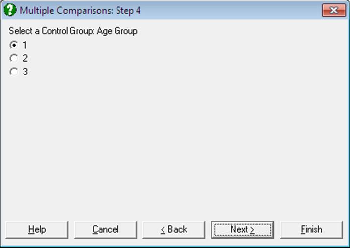
Two further dialogues pop up to select the control subgroup and the type of test.
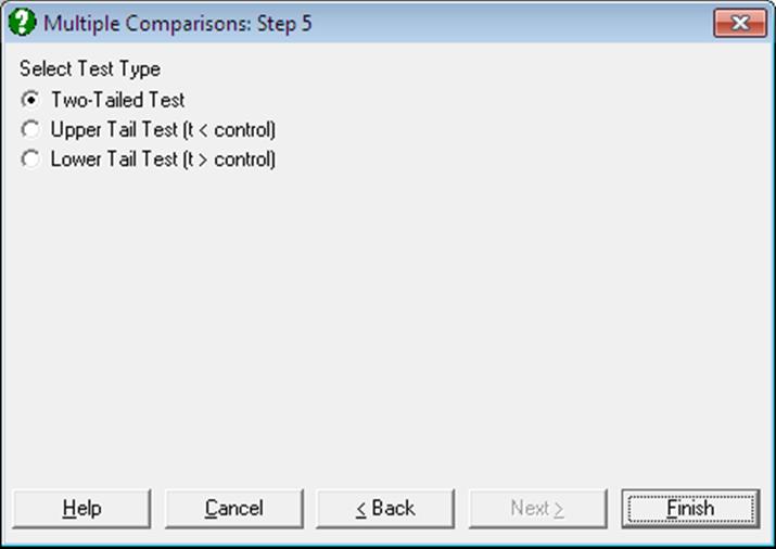
The type of test can be one of the following:
·
Two-tailed test: The null hypothesis µi = µctrl
is tested against µi ![]() µctrl
µctrl
·
Upper tail test: The null hypothesis µi < µctrl
is tested against µi ![]() µctrl
µctrl
·
Lower tail test: The null hypothesis µi > µctrl
is tested against µi ![]() µctrl
µctrl
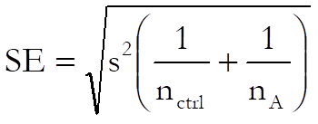
The standard error is calculated as:
Critical and p-values are computed using the algorithm developed by Charles Dunnett and the test can be performed at any confidence level. The maximum number groups (factor levels) is limited to 50. Critical and p-values generated by this algorithm are sensitive to difference in sample sizes. When all sample sizes are equal, the results are identical to the published tables for Dunnett’s critical values. When the sample sizes are not equal, the correct values may diverge from the published tables, as the latter do not take unequal sample size correction into consideration. By default, UNISTAT will compute the corrected critical values. You may, however, override this and not apply unequal sample size correction by including the following line in the [Options] section of Documents\Unistat10\Unistat10.ini file:
DunnettSampleSizeCorr=0
Example 1
Example 3-7 on p. 80 from Montgomery, D. C. (1991). Data from Example 3-1 is transformed into a suitable format first, where rows of the table are stacked in one column and a second factor column containing integers from 1 to 5 is created to keep track of the groups.
Open ANOTESTS, select Statistics 1 → Tests for ANOVA → Multiple Comparisons and select Cotton percentage (C15) [Factor] and Tensile strength (C16) as [Dependent]. Then select Dunnett, Arithmetic Mean of Sample Sizes from the next two dialogues and select group 5 as the control group from the last dialogue. Then select two-tailed test and accept the default Mean Square Error and Degrees of Freedom values. The following results will be obtained:
Multiple Comparisons
Dunnett
For Tensile strength, classified by Cotton percentage
Control Group: 5, Two-Tailed Test
Mean Square Error: 8.06, Degrees of Freedom: 20
** denotes significantly different pairs. Vertical bars show homogeneous subsets.
A pairwise test result is significant if its q stat value is greater than the table q.
|
Group |
Cases |
Mean |
5 |
|
|
1 |
5 |
9.8000 |
|
| |
|
5 |
5 |
10.8000 |
|
|| |
|
2 |
5 |
15.4000 |
|
| |
|
3 |
5 |
17.6000 |
** |
| |
|
4 |
5 |
21.6000 |
** |
| |
|
Comparison |
Difference |
Standard Error |
q Stat |
Table q |
Probability |
|
4 – 5 |
10.8000 |
1.7956 |
6.0149 |
2.6510 |
0.0000 |
|
3 – 5 |
6.8000 |
1.7956 |
3.7871 |
2.6510 |
0.0041 |
|
2 – 5 |
4.6000 |
1.7956 |
2.5619 |
2.6510 |
0.0600 |
|
1 – 5 |
-1.0000 |
1.7956 |
0.5569 |
2.6510 |
0.9469 |
|
Comparison |
Lower 95% |
Upper 95% |
Result |
|
4 – 5 |
6.0399 |
15.5601 |
** |
|
3 – 5 |
2.0399 |
11.5601 |
** |
|
2 – 5 |
-0.1601 |
9.3601 |
|
|
1 – 5 |
-5.7601 |
3.7601 |
|
|
Homogeneous Subsets: |
|
|
Group 1: |
1 5 |
|
Pooled mean = |
10.3000 |
|
95% Confidence Interval = |
8.4273 <> 12.1727 |
|
Group 2: |
5 2 |
|
Pooled mean = |
13.1000 |
|
95% Confidence Interval = |
11.2273 <> 14.9727 |
|
Group 3: |
3 |
|
Pooled mean = |
17.6000 |
|
95% Confidence Interval = |
14.9516 <> 20.2484 |
|
Group 4: |
4 |
|
Pooled mean = |
21.6000 |
|
95% Confidence Interval = |
18.9516 <> 24.2484 |
|
Between Homogeneous subsets: |
|
|
Group 2 – Group 1 |
|
|
Difference = |
2.8000 |
|
95% Confidence Interval = |
-2.5730 <> 8.1730 |
|
Group 3 – Group 2 |
|
|
Difference = |
4.5000 |
|
95% Confidence Interval = |
-2.0805 <> 11.0805 |
|
Group 4 – Group 3 |
|
|
Difference = |
4.0000 |
|
95% Confidence Interval = |
-3.5985 <> 11.5985 |
Example 2
Re-running the above example after including ComparisonCriterion=3 and ComparisonShortOutput=1 lines in Documents\Unistat10\Unistat10.ini file under the [Options] group, we obtain the following result.
Multiple Comparisons
Dunnett
|
Comparison |
Difference |
Lower 95% |
Upper 95% |
Result |
|
4 – 5 |
10.8000 |
6.0399 |
15.5601 |
** |
|
3 – 5 |
6.8000 |
2.0399 |
11.5601 |
** |
|
2 – 5 |
4.6000 |
-0.1601 |
9.3601 |
|
|
1 – 5 |
-1.0000 |
-5.7601 |
3.7601 |
|