7.4.2. Homogeneity of Variance Tests
One of the assumptions of the Analysis of Variance is that variances of the subgroups of data (defined by factor levels) are equal. Four tests are provided here to test whether this is the case. The null hypothesis tested is “all population variances are equal”, against the alternative hypothesis “all population variances are not equal”. If the null hypothesis is rejected, then it is possible to perform a number of multiple comparisons to determine which pairs of subgroups have significantly different variances.
The type of output depends on the number of factors selected. When a single factor variable is selected, a further Output Options Dialogue will allow you to perform multiple comparison tests for variances. If two or more factor variables are selected, then the Output Options Dialogue will not appear and the program will display the test results immediately.
7.4.2.1. Homogeneity of Variance Test Results
Five alternative test statistics are computed, and by default, all are reported on the same table. If more than one factor column is selected, an overall test is also performed on the subgroups defined by combinations of all levels in all factors. For instance, if two factors are selected, the test is performed on subgroups defined by two-way interactions. If you wish to see exactly which subgroups are tested, you can use the Table of Means procedure first. It is possible to control the statistics displayed in the output by including and editing the following line in the [Options] section of Documents\Unistat10\Unistat10.ini file:
HomoVariance=0
This parameter takes the following values:
-1: Overall test only
0: All five test statistics and the overall test (default)
1: Bartlett’s Chi-square Test
2: Bartlett-Box F test
3: Cochran’s C
4: Hartley’s F Test
5: Levene’s F Test
Bartlett’s Chi-Square Test
This is the original form of the homogeneity of variance test as introduced by Bartlett (see Zar, J. H. (2010), p. 220).
All subgroups of the dependent variable defined by the
selected factor are formed. Groups with a zero variance are omitted and the
counts (nj) and variances ![]() of the remaining groups are
determined. The test statistic is calculated as follows:
of the remaining groups are
determined. The test statistic is calculated as follows:
![]()
where m is the number of subgroups with non zero variances, n is the total number of cases within these subgroups and:
![]()
![]()
For a more accurate chi-square distribution the following term is computed:
![]()
and the modified test statistic is obtained as:
![]()
which is approximately chi-square distributed with m – 1 degrees of freedom.
As Bartlett’s chi-square test does not perform well when the population distributions are not normal, the following modification is widely regarded as a more powerful replacement.
Bartlett-Box F-test
The test statistic B is calculated as in Bartlett’s chi-square test, with the exception in the definition of:
![]()
and:
![]()
which is F-distributed with m – 1 and R degrees of freedom, where:
![]()
Cochran’s C
The test statistic is obtained by dividing the maximum subgroup variance by the sum of all subgroup variances.
![]()
An approximate tail probability is computed from the F-distribution:
![]()
with n/m – 1, (n/m – 1)(m – 1) degrees of freedom and it is multiplied by m.
Hartley’s F Test
The test statistic is obtained by dividing the maximum subgroup variance by the minimum subgroup variance.
![]()
A lookup table for critical values of Hartley’s F-values (Pearson & Hartley, 1954) is included for a limited range of degrees of freedom, number of subgroups and significance levels. The valid range is as follows:
·
4 ![]() degrees of freedom
degrees of freedom ![]() 10
10
· number of subgroups = 4, 6, 8, 9, 10, 12
· all subgroups have equal number of observations
· significance level = 0.05 or 0.01
The computed F-value is compared with the table value at 0.05 and 0.01 levels and the result is reported as:
· .0500 > if F > F.05
· .0100
> if F.05 ![]() F > F.01
F > F.01
·
.0100 < if F ![]() F.01
F.01
Levene’s F Test
This test has the advantage of being less sensitive to deviations from normality and is widely accepted as the most powerful homogeneity of variance test. The test statistic, which has an F distribution with (n – k) and (k – 1) degrees of freedom, is computed as follows:
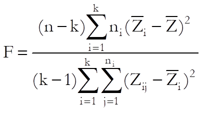
where:
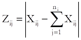
![]()
![]()
For a two sample version of this test see 6.1.1.6. Levene’s F-Test.
7.4.2.2. Multiple Comparisons Among Variances
This option is available only when a single factor variable is selected from the Variables Available list. If this is the case, a further dialogue will allow you to perform Tukey-HSD, Student-Newman-Keuls and Dunnett multiple comparison tests for variances.
For each test the q statistic is calculated as:
![]()
Tukey-HSD test for variances
All possible pairs are compared. Therefore, m(m – 1)/2 comparisons are made. The standard error is calculated as:
![]()
For details see 7.4.3.2. Tukey-HSD.
Student-Newman-Keuls test for variances
This test is identical to Tukey-HSD test except for the way the tabulated q values are computed.
For details see Student-Newman-Keuls.
Dunnett test for variances
This option will display two further dialogues, (1) selection of the control subgroup and (2) one or two-tailed test. All subgroups are compared with the control subgroup and therefore only M – 1 comparisons are made. The standard error is calculated as:
![]()
For details see 7.4.3.8. Dunnett test.
7.4.2.3. Homogeneity of Variance Examples
Example 1
Example 10.13 on p. 222 from Zar, J. H. (2010). The null hypothesis “all four feeds used have the same variance” is tested at a 95% confidence level.
The table format given in the book can be transformed into the factor format by using UNISTAT’s Data → Stack Columns procedure and the Level() function (see 3.4.2.5. Statistical Functions). All data should be stacked in a single column Weight and a factor column Feed created to keep track of the group memberships.
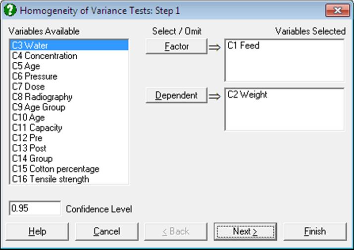
Open ANOTESTS, select Statistics 1 → Tests for ANOVA → Homogeneity of Variance Tests and select Feed (C1) as [Factor] and Weight (C2) as [Dependent] to obtain the following results:
Homogeneity of Variance Tests
For Weight
|
|
Test Statistic |
Probability |
|
classified by Feed |
|
|
|
Bartlett’s Chi-square Test |
0.4752 |
0.9243 |
|
Bartlett-Box F Test |
0.1610 |
0.9226 |
|
Cochran’s C (max var / sum var) |
0.3059 |
1.0000 |
|
Hartley’s F (max var / min var) |
1.9967 |
|
|
Levene’s F Test |
0.5816 |
0.6361 |
According to Bartlett’s chi-square test the tail probability is far greater than 5% and therefore the null hypothesis is not rejected. The probability value for Hartley’s F is not reported here, as this example does not fulfil the strict criteria outlined above.
Example 2
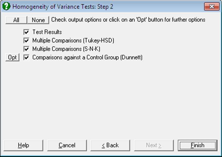
Running the above example after entering the HomoVariance=5 line in the [Options] section of Documents\Unistat10\Unistat10.ini file and selecting the Test Results and Comparisons against a Control Group (Dunnett) options only, the following output is obtained.
Homogeneity of Variance Tests
For Weight
|
|
Test statistic |
Probability |
|
classified by Feed |
|
|
|
Levene’s F Test |
0.0335 |
0.9914 |
Comparisons against a Control Group (Dunnett)
Method: 95% Dunnett interval.
Control Group: 1, Two-Tailed Test
** denotes significantly different pairs. Vertical bars show homogeneous subsets.
A pairwise test result is significant if its q stat value is greater than the table q.
|
Group |
N-1 |
Ln(variance) |
1 |
|
|
3 |
3 |
3.1342 |
|
| |
|
4 |
4 |
3.5131 |
|
| |
|
2 |
4 |
3.5340 |
|
| |
|
1 |
4 |
3.6262 |
|
| |
|
Comparison |
Difference |
Standard Error |
q Stat |
Table q |
Probability |
|
2 – 1 |
-0.0922 |
1.0000 |
0.0922 |
2.3533 |
0.9995 |
|
4 – 1 |
-0.1131 |
1.0000 |
0.1131 |
2.3533 |
0.9990 |
|
3 – 1 |
-0.4920 |
1.0801 |
0.4555 |
2.3533 |
0.9433 |
|
Comparison |
Lower 95% |
Upper 95% |
Result |
|
2 – 1 |
-2.4455 |
2.2611 |
|
|
4 – 1 |
-2.4663 |
2.2402 |
|
|
3 – 1 |
-3.0338 |
2.0499 |
|
|
Homogeneous Subsets: |
|
|
Group 1: |
3 4 2 1 |
Example 3
Open DEMODATA and select Statistics 1 → Descriptive Statistics → Homogeneity of Variance Tests and from the Variable Selection Dialogue select Output2 (C9) as [Variable] and Region (C10) and Type (C11) as [Factor]s. Selecting the Test Results output option and setting HomoVariance=-1 in Documents\Unistat10\Unistat10.ini file, the following output is obtained:
Homogeneity of Variance Tests
For Output2
|
|
Test statistic |
Probability |
|
classified by Region |
|
|
|
classified by Type |
|
|
|
Overall |
|
|
|
Bartlett’s Chi-square Test |
7.7995 |
0.1676 |
|
Bartlett-Box F Test |
1.5719 |
0.1648 |
|
Cochran’s C (max var / sum var) |
1.6238 |
0.8317 |
|
Hartley’s F (max var / min var) |
20.4095 |
|
|
Levene’s F Test |
1.3014 |
0.2777 |