7.3.0. Overview

As we have seen in Chapter 6, t-test is the appropriate procedure for testing whether two samples belong to the same population (where the null hypothesis tested is expressed as “H₀: μ₁ = μ₂”). When we need to test whether three (or more) samples belong to the same population (the null hypothesis “H₀: μ₁ = μ₂ = μ₃”), it may look as though performing a series of t-tests between all possible pairs of samples (the three null hypotheses “H₀: μ₁ = μ₂”, “H₀: μ₁ = μ₃” and “H₀: μ₂ = μ₃”), would solve the problem. Unfortunately this is not the case, since each t-test is associated with a confidence level (say 0.95) and when three are performed in a row, the final confidence level would drop to 0.95 x 0.95 x 0.95 = 0.86. Or in other words, the chance of rejecting the null hypothesis when it is in fact true (Type I error) would increase to 14%. As the number of samples to test increases, the chance of introducing an error would also increase. Analysis of Variance (ANOVA) was designed to overcome this problem by R A Fisher in 1920s.

The data for a simple ANOVA problem consists of a number of measurements taken from a number of different groups. An example would be the weights of a sample of five people from four different regions of the country. The criterion used in grouping (country) is called a factor and each group (North, South, East West) a level of the factor. If an ANOVA problem has only one factor, then it is called a one-way ANOVA. There may, however, be another factor defined on the same set of measurements, such as sex (a factor with two levels), which makes the problem a two-way ANOVA. In this case, we can compare the means of groups defined by each factor separately (the main effects) and also compare the means of groups defined by the combinations of the two factor levels (interactions), males in the North, females in the East, etc. In theory, there are no limits to the number of factors and the number of interactions that can be defined in an ANOVA design. ANOVA and GLM procedures assume that each factor has a maximum of 2000 levels, though this number may be increased by entering and editing the following line in Documents\Unistat60\Unistat60.ini file under the [Options] group:

   MaxFactorLevel=2000

Also see 3.2.12. Long String Table.

Let k be the number of groups and n_i the number of observations in group i for i = 1,…, k. in a one-way ANOVA problem. Let us also define the total number of observations as:

     

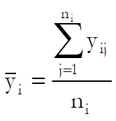
the mean of group i as:

     

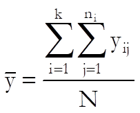
and the grand mean as:

     

If we express the deviation of an observation from the grand mean as the sum of its deviation from its own group mean (within-group) plus the deviation of its group mean from the grand mean (between-group) we have:

     

If we then take the squares of both sides, sum over i and j and rearrange, we obtain:

     

In other words:

      Total Ssq = Within-Groups Ssq + Between-Groups Ssq

where Ssq stands for sum of squares.

Our aim is to test the null hypothesis that “all means are equal”. Therefore, the entity we are interested in is the Between-Groups Ssq. Since the Within-Groups Ssq term represents the rest of variation in data, we can also call it the Error Term. We construct the ANOVA table as follows:

 

	Sum of Squares (Ssq)	Degrees of Freedom	Mean Squares (MSQ)	F-Statistic	Probability
Factor	Between-Groups Ssq	k - 1	Between-Groups Ssq / (k - 1)	Between-Groups MSQ / Within-Groups MSQ	P-value for F(k-1)(N-k)
Error	Within-Groups Ssq	N - k	Within-Groups Ssq / (N - k)
Total	Total Ssq	N - 1	Total Ssq / (N - 1)

 

The F-statistic for the Factor is the test statistic. The associated one-tail probability from the F-distribution is calculated with (k ‑ 1) and (N ‑ k) degrees of freedom and it is reported in the last column of the ANOVA table. If this p‑value is less than or equal to a given confidence level (usually 5%), then we reject the null hypothesis “H₀: μ₁ = μ₂ =…= μ_k”, or in other words, we conclude that the k samples tested do not belong to the same population.

Note that all we can conclude using ANOVA is whether the k population means are all equal or not. If they are not equal, then ANOVA does not tell us which ones are different. In order to find out which pairs or groups of population means are different, one of the Multiple Comparisons tests should be used. If the ANOVA design is more complicated than one‑way, then the General Linear Model procedure may also be used to find out the significantly different groups (see 7.3.2.3. GLM Output Options).

7.3.0.1. ANOVA and GLM Data Format

In order to analyse ANOVA and GLM designs in a general purpose statistical program, the data should be organised in an accurate and logical way. The approach adopted in almost all serious statistical packages involves stacking all measurement data (the explanatory variable) in a single column, and expressing the various group memberships of these observations in separate corresponding categorical data columns (factors). The user will often face the problem of having to convert a published data table into this format.

For instance, consider the Randomised Block Designs ANOVA example given in Table 5-4 p. 140 by Montgomery, D. C. (1991). Measurements on Hardness are given in the following format:

 

	Coupon (Block)
Type of Tip	1	2	3	4
1	-2	-1	1	5
2	-1	-2	3	4
3	-3	-1	0	2
4	2	1	5	7

 

This should be entered into UNISTAT as follows:

 

Hardness	Tip	Coupon
-2	1	1
-1	1	2
1	1	3
5	1	4
-1	2	1
-2	2	2
3	2	3
4	2	4
-3	3	1
-1	3	2
0	3	3
2	3	4
2	4	1
1	4	2
5	4	3
7	4	4

 

If the data has already been entered into a spreadsheet in the form of a table, you do not have to retype it in the above format manually. UNISTAT’s own spreadsheet Data Processor provides a number of functions that will help you to do the transformation automatically. The Data → Stack Columns procedure can be used to stack the hardness measurements in a column and create the Tip column automatically (see 3.3.9. Stack Columns).

You may also use the function Level() which is designed to generate factor columns containing regular (balanced) levels automatically (see 3.4.2.5. Statistical Functions). To do this, first create the data column and then enter the function Level(4);B in a blank column (to create the Tip column) and Level(4) into the next blank column (to create the Coupon column).

For the analysis, select Tip and Coupon as [Factor]s and Hardness as [Dependent].

Let us also consider a more complex example known as Graeco Latin Squares Designs given in Table 5-20 p. 168 by Montgomery, D. C. (1991).

 

Batches of Raw	Operators
Material	1	2	3	4	5
1	Aα = -1	Bc = -5	Ce = -6	Db = -1	Ed = -1
2	Bb = -8	Cd = -1	Dα = 5	Eχ = 2	Ae = 11
3	Cc = -7	De = 13	Eb = 1	Ad = 2	Bα = -4
4	Dd = 1	Eα = 6	Ac = 1	Be = -2	Cb = -3
5	Ee = -3	Ab = 5	Bd = -5	Cα = 4	Dc = 6

This table is entered into UNISTAT as follows:

 

Operator	Batch	Formulation	Test assemblies	Coded Data
1	1	A	a	-1
2	1	B	c	-5
3	1	C	e	-6
4	1	D	b	-1
5	1	E	d	-1
1	2	B	b	-8
2	2	C	d	-1
3	2	D	a	5
4	2	E	c	2
5	2	A	e	11
1	3	C	c	-7
2	3	D	e	13
3	3	E	b	1
4	3	A	d	2
5	3	B	a	-4
1	4	D	d	1
2	4	E	a	6
3	4	A	c	1
4	4	B	e	-2
5	4	C	b	-3
1	5	E	e	-3
2	5	A	b	5
3	5	B	d	-5
4	5	C	a	4
5	5	D	c	6

 

where Formulation, Batch, Operator and Test assemblies are the factors and Coded Data is the dependent variable.

7.3.0.2. ANOVA Designs

It is possible to test a large number of experimental designs using UNISTAT’s Analysis of Variance and GLM procedures. In this section we shall describe seven major designs and demonstrate how we can solve these problems using UNISTAT with the help of published examples.

7.3.0.2.1. Randomised Block Designs

In many ANOVA problems, it is desirable to control the variability from known nuisance factors (blocks). We want to remove this variability from the error sum of squares to increase the power of the test. For example if we wish to determine the effectiveness of different fertilisers on a particular crop, we might try each fertiliser on the crop in a number of different fields. But the soil in each field might not be of the same quality and this would add variability to the results. As a result, the experimental error will reflect both the random error and the variability between fields. A better design would be the randomised block design, where each fertiliser is tested in each field. A randomised block design is said to be complete if all the treatments are used in all the blocks.

 

	Block 1		Block 2		Block b
Treatment 1	y11		y12	…	y1b
Treatment 2	y21		y22	…	y2b
	.		.		.
	.		.		.
Treatment a	ya1		ya2	…	yab

 

These designs can be constructed in UNISTAT using one of ANOVA or GLM procedures.

Example

Table 5-4 on p. 140 from Montgomery, D. C. (1991). The table format given in the book can be transformed into the factor format by using UNISTAT’s Data → Stack Columns procedure and the Level() function (see 3.4.2.5. Statistical Functions). All data should be stacked in a single column Hardness and two factor columns Tip and Coupon created to keep track of the group memberships. Therefore, the resulting data matrix should have 16 rows and 3 columns.

Open ANOVA, select Statistics 1 → ANOVA and GLM → Analysis of Variance, and select Tip (C2) and Coupon (C3) as [Factor]s and Hardness (C1) as [Dependent]. Then select Classic Experimental Approach and no interaction terms to obtain the following ANOVA table:

Analysis of Variance

Approach: Classic Experimental

Dependent variable: Hardness

 

Due To	Sum of Squares	DoF	Mean Square	F-stat	Probability
Main Effects	121.000	6	20.167	22.688	0.0001
Tip	38.500	3	12.833	14.438	0.0009
Coupon	82.500	3	27.500	30.938	0.0000
Explained	121.000	6	20.167	22.688	0.0001
Error	8.000	9	0.889
Total	129.000	15	8.600

 

The result is the F-statistic and its probability value for Tip. Since the probability 0.0009 is much smaller than 5%, we reject the null hypothesis and conclude that the means differ significantly. In other words, the conclusion is that the type of tip affects the hardness values. The F-statistic and its probability for Coupon is not strictly meaningful, but informally we can see that the Coupon were an important source of variation in the resulting hardness, and power of the analysis has been increased by using a Randomised Block Designs.

7.3.0.2.2. Repeated Measures Designs

It is often the case that repeated measurements are taken on the same subject. This typically happens when the subjects are people and measurements are taken from the same people at different times, following a particular treatment.

If the subject receives different treatments and the treatments are administered in a random order, then it is possible to regard the experiment as having a Randomised Block Designs with the subject as a blocking factor. If the subject receives different treatments in a specified order, then it is possible to regard the experiment as a Crossover Designs. If each subject receives the same treatment a number of times, this should be considered as a repeated measures design.

In a repeated measures design, the total sum of squares can be partitioned into the Between Subjects sum of squares and the Within Subjects sum of squares. It is assumed that these terms are statistically independent. This means that the residual sum of squares can also be partitioned into Error Between Subjects and Error Within Subjects. These terms can be used to find the various factor F-ratios to increase the power of the analysis.

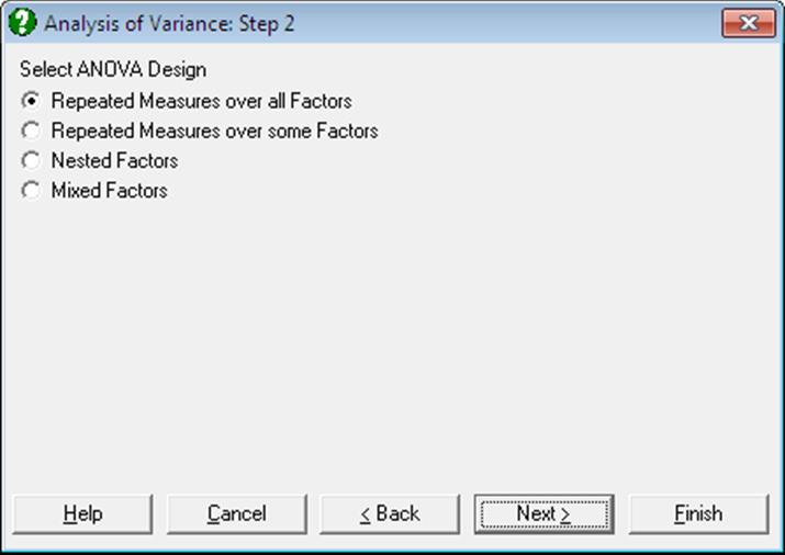
7.3.0.2.2.1. Repeated Measures over all Factors

This is the case when each subject only receives one level of each factor. The two-factor experiment of this kind is shown schematically below.

 

		c1	c2	L	cr
	b1	X111	X112	L	X11r
a1	M	M	M		M
	bq	X1q1	X1q2	L	X1qr
M	M
	b1	Xp11	Xp12	L	Xp1r
ap	M	M	M		M
	bq	Xpq1	Xpq2	L	Xpqr

 

Each row represents a group of subjects and each subject is measured on r occasions. This means that the factors A and B sum of squares are contained in the Between Subjects sum of squares. Only the Trial (factor C) sum of squares is contained in the Within Subjects sum of squares.

This can be done using the Analysis of Variance (ANOVA) procedure and selecting the Repeated Measures over all Factors option or using the General Linear Model (GLM). In order to use the GLM procedure, an additional factor column must be created in the spreadsheet to give information about the repeated measure (the Trial factor). In ANOVA with Repeated Measures over all Factors, this additional factor is created internally by the program, assuming a repeated measure across all the factors.

Example 1: Using ANOVA with Repeated Measures over all Factors

Table 7.4-3 on p. 341 from Winer, B. J. (1970). The table format given in the book can be transformed into the factor format by using UNISTAT’s Data → Stack Columns procedure and the Level() function (see 3.4.2.5. Statistical Functions). All data should be stacked in a single column Score and three factor columns created Subject, Anxiety and Tension.

Open ANOVA and select Statistics 1 → ANOVA and GLM → Analysis of Variance. Select Score (C24) as [Dependent], Subject (C23) as [Repeated], Anxiety (C21) and Tension (C22) as [Factor]s. From the next two dialogues select the Repeated Measures over all Factors and Classic

Analysis of Variance

Design: Repeated Measures over all Factors

Approach: Classic Experimental

Dependent Variable: Score

 

Due To	Sum of Squares	DoF	Mean Square	F-Stat	Prob
Between Subjects	181.000	11	16.455
Anxiety	10.083	1	10.083	0.978	0.3517
Tension	8.333	1	8.333	0.808	0.3949
Anxiety × Tension	80.083	1	80.083	7.766	0.0237
Error Between	82.500	8	10.313
Within Subjects	1077.000	36	29.917
Trial	991.500	3	330.500	152.051	0.0000
Anxiety × Trial	8.417	3	2.806	1.291	0.3003
Tension × Trial	12.167	3	4.056	1.866	0.1624
Anxiety × Tension × Trial	12.750	3	4.250	1.955	0.1477
Error Within	52.167	24	2.174
Total	1258.000	47	26.76596

 

Example 2: Using General Linear Model

To use the GLM procedure with this example, an extra factor column Trial must be created. This is defined as the number of times a measurement is made on a particular subject. So the second measurement taken with subject i would result in a 2 in the Trial column, the third measurement with subject j would results in a 3 in the Trial column, etc.

 

Anxiety	Tension	Subject	Trial
1	1	1	1
1	2	1	2
2	1	1	3
2	2	1	4
1	1	2	1
1	2	2	2
2	1	2	3
2	2	2	4

 

So the two factors, Anxiety and Tension play no part in the calculation of the Trial column.

Open ANOVA and select Statistics 1 → ANOVA and GLM → General Linear Model. Select Score (C24) as [Dependent], Subject (C23) as [Repeated]. Select the following terms as factors, and at the following dialogue select the F-Statistic denominators as shown.

 

C21 Anxiety	Error Between C23 Subject
C22 Tension	Error Between C23 Subject
C21 Anxiety × C22 Tension	Error Between C23 Subject
C25 Trial	Error Within C23 Subject
C21 Anxiety × C25 Trial	Error Within C23 Subject
C22 Tension × C25 Trial	Error Within C23 Subject
C21 Anxiety × C22 Tension × C25 Trial	Error Within C23 Subject

 

From the Output Options Dialogue select only the ANOVA option to obtain the following results.

General Linear Model

ANOVA

Dependent Variable: Score

 

Due To	Sum of Squares	DoF	Mean Square	F-Stat		Prob
Constant	4800.000	1	4800.000	35.644		0.0000
Between Subjects	181.000	11	16.455
Anxiety	10.083	1	10.083	0.978	a	0.3517
Tension	8.333	1	8.333	0.808	a	0.3949
Anxiety × Tension	80.083	1	80.083	7.766	a	0.0237
Error Between	82.500	8	10.313
Within Subjects	1077.000	36	29.917
Trial	991.500	3	330.500	152.051	b	0.0000
Anxiety × Trial	8.417	3	2.806	1.291	b	0.3003
Tension × Trial	12.167	3	4.056	1.866	b	0.1624
Anxiety × Tension × Trial	12.750	3	4.250	1.955	b	0.1477
Error Within	52.167	24	2.174
Explained	1123.333	15	74.889	17.795		0.0000
Error	134.667	32	4.208
Total	1258.000	47	26.766

 

R-squared =	0.8930
Adjusted R-squared =	0.8428

a F-Statistic: Error Between

b F-Statistic: Error Within

In this particular example, ANOVA with the Repeated Measures over all Factors option and GLM produce exactly the same results. This would not always be the case since GLM always adopts the Regression Approach and with ANOVA you can select different approaches. However with a balanced design (as above) all three approaches will give the same result.

7.3.0.2.2.2. Repeated Measures over some Factors

This is the case when each subject receives only one level of some factors but all levels of other factors. The three-factor experiment of this kind is shown schematically below.

 

		b1		L		bq
	c1	L	cr	L	c1	L	cr
a1	X111	L	X11r	L	X1q1		X1qr
a2	X211	L	X21r	L	X2q1		X2qr
M	M		M		M		M
ap	Xp11	L	Xp1r	L	Xpq1		Xpqr

 

Each row represents a group of subjects and each subject only receives one level of factor A. However each subject receives all levels of factors B and C. This means that only the factor A sum of squares is contained in the Between Subjects sum of squares. The factor B and C sum of squares is contained in the Within Subjects sum of squares.

Example

Table 7.3-3 on p. 324 from Winer, B. J. (1970). The table format given in the book can be transformed into the factor format by using UNISTAT’s Data → Stack Columns procedure and the Level() function (see 3.4.2.5. Statistical Functions). All data should be stacked in a single column Score and five factor columns created Subject, Noise, Period, Dial and SubjWGrps.

The artificial factor SubjWGrps has been set up to partition the Error Within Subjects, and these partitions are used for the F-statistic ratios in this example. The factor SubjWGrps is equivalent to Subject(Noise) nest term. However since terms of the form FactorA × FactorB(FactorC) can not be specified, SubjWGrps needs to be built explicitly. The table below shows how this is done. Note that each combination of Subject and Noise results in a different level. However, when each level of Noise is met for the first time this is pooled into level 0.

 

Subject	Noise	Count	SubjWGrps
1	High	1	0
2	High	2	2
3	High	3	3
4	Low	4	0
5	Low	5	5
6	Low	6	6

 

The SubjWGrps column calculated here has nothing to do with the Trial column calculated in the previous example (see 7.3.0.2.2.1. Repeated Measures over all Factors). In fact it can informally be considered as the opposite of the Trial column from the previous example.

Open ANOVA and select Statistics 1 → ANOVA and GLM → General Linear Model. Select Score (C26) as [Dependent] and Subject (C27) as [Repeated]. Select the following terms as factors, and on the following dialogue select the F-statistic denominators as shown.

 

C30 Noise	Error Between C27 Subject
C29 Period	C29 Period × C31 SubjWGrps
C29 Period × C30 Noise	C29 Period × C31 SubjWGrps
C29 Period × C31 SubjWGrps	Error Term
C28 Dial	C28 Dial × C31 SubjWGrps
C28 Dial × C30 Noise	C28 Dial × C31 SubjWGrps
C28 Dial × C31 SubjWGrps	Error Term
C28 Dial × C29 Period	C28 Dial × C29 Period × C31 SubjWGrps
C28 Dial × C29 Period × C30 Noise	C28 Dial × C29 Period × C31 SubjWGrps
C28 Dial × C29 Period × C31 SubjWGrps	Error Term

 

The following results are obtained:

General Linear Model

ANOVA

Dependent Variable: Score

 

Due To	Sum of Squares	DoF	Mean Square	F-Stat		Prob
Constant	105868.167	1	105868.167	35.782		0.0000
Between Subjects	2959.278	5	591.856
Noise	468.167	1	468.167	0.751	a	0.4348
Error Between	2491.111	4	622.778
Within Subjects	6965.556	48	145.116
Period	3722.333	2	1861.167	63.389	b	0.0000
Period × Noise	333.000	2	166.500	5.671	b	0.0293
Dial	2370.333	2	1185.167	89.823	c	0.0000
Dial × Noise	50.333	2	25.167	1.907	c	0.2102
Dial × Period	10.667	4	2.667	0.336	d	0.8499
Dial × Period × Noise	11.333	4	2.833	0.357	d	0.8357
Error Within	467.556	32	14.611
Period × SubjWGrps	234.889	8	29.361
Dial × SubjWGrps	105.556	8	13.194
Dial × Period × SubjWGrps	127.111	16	7.944
Explained	6966.167	17	409.775	4.986		0.0000
Error	2958.667	36	82.185
Total	9924.833	53	187.261

a F-Statistic: Error Between

b F-Statistic: Period × SubjWGrps

c F-Statistic: Dial × SubjWGrps

d F-Statistic: Dial × Period × SubjWGrps

 

The Between Subjects sum of squares and the Within Subjects sum of squares partition the Total sum of squares. The Error Between and the Error Within partition the Total Error sum of squares. And the Period × SubjWGrps, Dial × SubjWGrps and Dial × Period × SubjWGrps errors partition the Error Within.

So, in the example output above, Period × SubjWGrps, Dial × SubjWGrps and Dial × Period × SubjWGrps class="UniDialog">Between Subjects. The terms Period, Period × Noise, Dial, Dial × Noise, Dial × Period, and Dial × Period × Noise are Within Subjects. All the Between Subjects and

7.3.0.2.3. Latin Squares Designs

Consider an experiment to compare k treatments in which there are two nuisance factors (blocks) each at k levels (this is more common than it sounds). A complete factorial design with one observation at each level would need k³ observations, but a Latin Square needs only k-Squared observations. Consider the following design with k = 5. The treatments are A, B, C, D and E, the two other sources of variation are represented by the rows and columns of the table.

 

	Column
Row	1	2	3	4	5
1	A	B	C	D	E
2	E	A	B	C	D
3	D	E	A	B	C
4	C	D	E	A	B
5	B	C	D	E	A

 

Only k-Squared (= 25) observations are made, since at each combination of a row and a column only one of the five treatments is used. Each treatment occurs in each row and column precisely once. It is assumed that there are no interactions between the three factors.

These designs are constructed in UNISTAT using the ANOVA procedure. Treatment, columns and rows are selected as factors and all interaction terms are omitted. The main result is the F-statistic on the treatment.

Example

Table 5-11 on p. 159 from Montgomery, D. C. (1991). The table format given in the book can be transformed into the factor format by using UNISTAT’s Data → Stack Columns procedure and the Level() function (see 3.4.2.5. Statistical Functions). All data should be stacked in a single column Coded Data and three factor columns Operator, Batch and Formulation created to keep track of the group memberships.

Open ANOVA and select Statistics 1 → ANOVA and GLM → Analysis of Variance, Operator (C4), Batch (C5) and Formulation (C6) as [Factor]s and Coded Data (C7) as [Dependent]. Then select Classic Experimental Approach and omit all interaction terms to obtain the following ANOVA table:

Analysis of Variance

Approach: Classic Experimental

Dependent Variable: Coded Data

 

Due To	Sum of Squares	DoF	Mean Square	F-Stat	Prob
Main Effects	548.000	12	45.667	4.281	0.0089
Operator	150.000	4	37.500	3.516	0.0404
Batch	68.000	4	17.000	1.594	0.2391
Formulation	330.000	4	82.500	7.734	0.0025
Explained	548.000	12	45.667	4.281	0.0089
Error	128.000	12	10.667
Total	676.000	24	28.167

 

The result is the Formulation F-statistic and its tail probability. The Batch and Operator variables are nuisance factors (blocks) which are removed from the error sum of squares to increase the power of the test. The F-statistic and probability for Batch and Operator are not strictly meaningful, but informally we can see that the power of the test has been increased by including them in the design.

7.3.0.2.4. Graeco Latin Squares Designs

Consider a Latin square design with another factor added. Denote the levels of this extra factor by Greek letters. If each Latin letter appears once and only once with each Greek letter then the design is called a Graeco-Latin square.

 

	Column
Row	1	2	3	4
1	Aα	Bb	Cc	Dd
2	Bd	Ac	Db	Cα
3	Cb	Dα	Ad	Bc
4	Dc	Cd	Bα	Ab

 

A Graeco-Latin square design exists for all k ≥ 3 except for k = 6. The Graeco-Latin square design allows investigation of four factors (rows, columns, Latin letters and Greek letters), each at k levels with only k-Squared observations.

These designs are constructed in UNISTAT using ANOVA. Selecting the Latin letters, Greek letters, columns and rows as factors. All interaction terms are omitted. The main result is the F-statistic on the Latin letters.

Example

Table 5-20 on p. 168 from Montgomery, D. C. (1991). The table format given in the book can be transformed into the factor format by using UNISTAT’s Data → Stack Columns procedure and the Level() function (see 3.4.2.5. Statistical Functions). All data should be stacked in a single column Coded Data and four factor columns Operator, Batch, Formulation and Test created to keep track of the group memberships.

Open ANOVA, select Statistics 1 → ANOVA and GLM → Analysis of Variance, select Operator (C4), Batch (C5), Formulation (C6) and Test assemblies (C8) as [Factor]s and Coded Data (C7) as [Dependent]. Then select Classic Experimental Approach and no interaction terms (the default) to obtain the following ANOVA table:

Analysis of Variance

Approach: Classic Experimental

Dependent Variable: Coded Data

 

Due To	Sum of Squares	DoF	Mean Square	F-Stat	Prob
Main Effects	610.000	16	38.125	4.621	0.0171
Operator	150.000	4	37.500	4.545	0.0329
Batch	68.000	4	17.000	2.061	0.1783
Formulation	330.000	4	82.500	10.000	0.0033
Test assemblies	62.000	4	15.500	1.879	0.2076
Explained	610.000	16	38.125	4.621	0.0171
Error	66.000	8	8.250
Total	676.000	24	28.167

 

The result is the Formulation F-statistic and its probability. The Batch, Operator and Test assemblies variables are nuisance factors (blocks) which are removed from the error sum of squares to increase the power of the test. The F-statistic and its probability for Batch, Operator and Test assemblies are not strictly meaningful, but informally we can see that the power of the test has been increased by including them in the design.

7.3.0.2.5. Split-Plot Designs

In some experimental designs, one of the factors may be a sub-unit of another factor. For example a field may be divided into main plots and these main plots split into sub plots. If one factor is allocated to the main plots and another factor to their sub plots, then we have a Split-Plot design. The sub plots factor is compared against the variation between sub plots, the main plots factor is compared against the variation between the main plots. The variation within the main plots (between the sub plots) is likely to be less than the variation between the main plots. So the sub plots factor is tested with more power. The main plots factor is said to be confounded with blocks.

These designs are also called split-unit designs, in which case the terms main units and sub units are used instead of main plots and sub plots. Some examples of main plots and sub plots are as follows:

 

Main Plot	Sub Plot
Days	Hours within day
Subject	Occasion with the subject
Field	Area within the field

 

These designs are constructed in UNISTAT using ANOVA with the Repeated Measures over some Factors option. Select the main plot as the first factor and the sub plot as the first repeated measure.

Example

Example 8.13 on p. 270 from Armitage, P. & G. Berry (1994). The table format given in the book can be transformed into the factor format by using UNISTAT’s Data → Stack Columns procedure and the Level() function (see 3.4.2.5. Statistical Functions). All data should be stacked in a single column Swabs and three factor columns Crowding, Status and Family created to keep track of the group memberships.

Open ANOVA, select Statistics 1 → ANOVA and GLM → Analysis of Variance and select Crowding (C9) and Status (C10) as [Factor]s, Family (C11) as [Repeated] and Swabs (C12) as [Dependent]. From the next two dialogues select the Repeated Measures over some Factors and Classic Experimental Approach options. At the interaction terms dialogue check the only interaction term Crowding × Status to obtain the following ANOVA table:

Analysis of Variance

Design: Repeated Measures over some Factors

Approach: Classic Experimental

Dependent Variable: Swabs

 

Due To	Sum of Squares	DoF	Mean Square	F-Stat	Prob
Main Effects	2004.156	6	334.026	13.214	0.0000
Crowding	470.489	2	235.244	5.223	0.0190
Error (Family)	675.600	15	45.040
Status	1533.667	4	383.417	15.167	0.0000
2 Way Interactions	72.400	8	9.050	0.358	0.9384
Crowding × Status	72.400	8	9.050	0.358	0.9384
Explained	2076.556	14	148.325	5.868	0.0000
Error	1516.733	60	25.279
Total	4268.889	89	47.965

 

Crowding is compared against the between family variation instead of the overall error term. This increases the power of the test on the Crowding effect. The interaction between Crowding and Status is not significant, so we might consider removing it from the model.

7.3.0.2.6. Nested Designs

Consider an experiment where the levels of one factor (child) are different depending on the level of another factor (parent). For example the parent factor may be Country and the child factor Region. The north of England is not related to the north of Germany and thus Region is a nested factor of Country.

Nested designs resemble factorial designs with certain cells missing. This is because one factor is nested under another so that not all combinations of the two factors are observed.

These designs are constructed in UNISTAT using ANOVA selecting the parent as a factor and the child as the corresponding repeated measure. Then the Nested Factors option is selected from the next dialogue.

Example

Table 13-3 on p. 443 from Montgomery, D. C. (1991). The table format given in the book can be transformed into the factor format by using UNISTAT’s Data → Stack Columns procedure and the Level() function (see 3.4.2.5. Statistical Functions). All data should be stacked in a single column Purity and two factor columns Supplier and Batches created to keep track of the group memberships.

Open ANOVA and select Statistics 1 → ANOVA and GLM → Analysis of Variance. Select Supplier (C13) as [Factor], Batches (C14) as [Repeated] and Purity (C15) as [Dependent]. Then select Nested Factors and Classic Experimental Approach from the next two dialogues to obtain the following results:

Analysis of Variance

Design: Nested Factors

Approach: Classic Experimental

Dependent Variable: Purity

 

Due To	Sum of Squares	DoF	Mean Square	F-Stat	Prob
Main Effects	84.972	11	7.725	2.927	0.0135
Supplier	15.056	2	7.528	2.853	0.0774
Batches(Supplier)	69.917	9	7.769	2.944	0.0167
Explained	84.972	11	7.725	2.927	0.0135
Error	63.333	24	2.639
Total	148.306	35	4.237

 

We conclude that the difference between Batches is a source of variation.

7.3.0.2.7. Crossover Designs

Crossover Designs occur when subjects are reused, typically in time. For instance, in an experiment designed to compare the effects of drugs A and B, half the sample (chosen at random) take drug A and the remaining half take drug B at the start of the experiment. Some time later the first sample now take drug B and the second sample take drug A. It is important that effect of the first drug taken does not carryover and affect the performance of the second drug taken. If this does happen it is called the carryover effect.

In UNISTAT the crossover design is analysed in two steps. The first step tests whether the carryover effect is significant. If the carryover effect is not significant then a standard ANOVA can be used on the remaining factors. If the carryover effect is significant then analysis should be restricted to the first trial, and in future experiments a larger time period left between the trials.

The significance of the carryover effect is tested using a Split-Plot design (see 7.3.0.2.5. Split-Plot Designs) of the treatment order against the subjects. To do this a factor column needs to be created which represents the order in which the treatments were given. The easiest way to do this is to have a string column with characters representing each treatment in the order they were given, say, for 3 treatments A, B and C. The column would contain ABC, ACB, BAC, BCA, CAB and CBA as required. When this sequence factor column is defined, it will be selected as the first factor and the subjects as a repeated measure. The sequence should not be significant. If it is not, continue to analyse the full data. If it is significant, then it may only be possible to use the results from the first trial.

Example

Table 11.5 on p. 380 from Bolton, S. (1990). The table format given in the book can be transformed into the factor format by using UNISTAT’s Data → Stack Columns procedure and the Level() function (see 3.4.2.5. Statistical Functions). All data should be stacked in a single column AUC and four factor columns Period, Subject, Sequence and Treatment created to keep track of the group memberships.

The first step is to test for any carryover (Sequence) effects. This is a Split-Plot design (see 7.3.0.2.5. Split-Plot Designs), with Sequence against Subject. Open ANOVA and select Statistics 1 → ANOVA and GLM → Analysis of Variance. Select Sequence (C18) as [Factor], Subject (C17) as [Repeated] and AUC (C20) as [Dependent]. Then select the Repeated Measures over some Factors and Classic Experimental Approach options to obtain the following ANOVA table:

Analysis of Variance

Design: Repeated Measures over some Factors

Approach: Classic Experimental

Dependent Variable: AUC

 

Due To	Sum of Squares	DoF	Mean Square	F-Stat	Prob
Main Effects	4620.375	1	4620.375	1.590	0.2313
Sequence	4620.375	1	4620.375	1.187	0.3016
Error(Subject)	38940.083	10	3894.008
Explained	4620.375	1	4620.375	1.590	0.2313
Error	34870.500	12	2905.875
Total	78430.958	23	3410.042

 

The critical value is the F-statistic and its probability for Sequence. This shows that the sequence is not significant, so there are no significant crossover effects in the data. We can then proceed to analyse the full data set. This is done by selecting ANOVA and Subject (C17), Period (C16) and Treatment (C19) as [Factor]s and AUC (C20) as [Dependent]. Select Classic Experimental Approach and no interaction terms:

Analysis of Variance

Approach: Classic Experimental

Dependent Variable: AUC

 

Due To	Sum of Squares	DoF	Mean Square	F-Stat	Prob
Main Effects	67760.875	13	5212.375	4.885	0.0083
Subject	43560.458	11	3960.042	3.711	0.0240
Period	13490.042	1	13490.042	12.643	0.0052
Treatment	10710.375	1	10710.375	10.038	0.0100
Explained	67760.875	13	5212.375	4.885	0.0083
Error	10670.083	10	1067.008
Total	78430.958	23	3410.042

 

This shows that Subject, Period and Treatment are all significant.