10.1. Parallel Line Method
Balanced, symmetric or unbalanced assays can be analysed. The analysis is based on a regression of the response variable against the natural logarithm of the dose variable. A separate line is fitted on each preparation, subject to a constraint that they should be parallel. An assay is said to be balanced when:
1) there is an equal number of cases in each treatment group,
2) there is an equal number of dose groups for each preparation and
3) successive dose levels are the same for all preparations.
An assay fulfilling the first two conditions but having different dose levels for different preparations (yet having the same ratio of successive dose levels) will be called symmetric. Assays not fulfilling one or more of these conditions will be called asymmetric or unbalanced.
For validity tests, the following Analysis of Variance (ANOVA) options are available:
1) Completely randomised design
2) Randomised block design
3) Latin square design
4) Twin and triple crossover designs
The unbalanced assays can only be analysed using the Completely Randomised Design option. All other options require symmetric or balanced assays. In most cases, the program will detect whether an assay is unbalanced, symmetric or balanced and apply the relevant algorithm automatically.
Note that the example data sets given in European Pharmacopoeia (1997-2017) Parallel Line Method are all balanced.
10.1.1. Parallel Line Variable Selection
Once the data is arranged as described above (see section 10.0.1. Data Preparation), select Bioassay → Parallel Line Method from UNISTAT menus. A Variable Selection Dialogue will pop up.
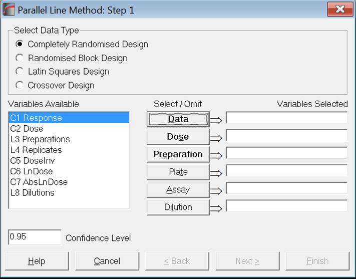
Data columns available for selection are listed on the left. Variables are referred to by their column numbers, which are prefixed by a single letter representing the type of data. For instance, in the above example C1, C2 and C4 are numeric columns, whereas L3 means that column three contains Long Strings. Columns containing Short Strings (up to 8 characters) are prefixed by (S). Other data types that will probably not be used in bioassays are date (D) and time (T). If Column Labels have been entered, they will also appear in the list next to the column numbers.
You will need to assign tasks to variables by sending them to boxes on the right. To do this, highlight the variable on the left list and click on the desired task button (i.e. one of the command buttons in the middle of the dialogue). Likewise, you can deselect an already selected variable by highlighting it on the right list first and then clicking its task button.
Designs can be unbalanced, i.e. the number of replicates for each dose-preparation combination may be different, dose levels for standard and test preparations may be different, there can be more than one test preparation, but the first five characters of the standard preparation label should be “stand” or “refer” in any language (capitalisation is not significant). Otherwise the first preparation encountered in the [Preparation] column will be considered as the standard. It is compulsory to select at least three variables [Data], [Dose] and [Preparation], which have bold button fonts. There are three optional variables [Plate], [Assay] and [Dilution]. A plate effect, that will be subtracted from the residual sum of squares, can be calculated if required. For the latter two options see sections 10.0.4. Multiple Assays with Combination and 10.0.2. Doses, Dilutions and Potency respectively. Note that if the design is balanced, the plate effect will generate the same results as Randomised Block Design.
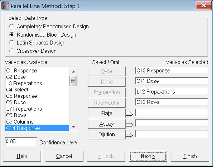
The frame Select Data Type (at the top) displays options for the type of Analysis of Variance to be performed. The number of variables to be selected is different for these types of analyses. When the second option Randomised Block Design is selected, four compulsory variables will need to be selected.
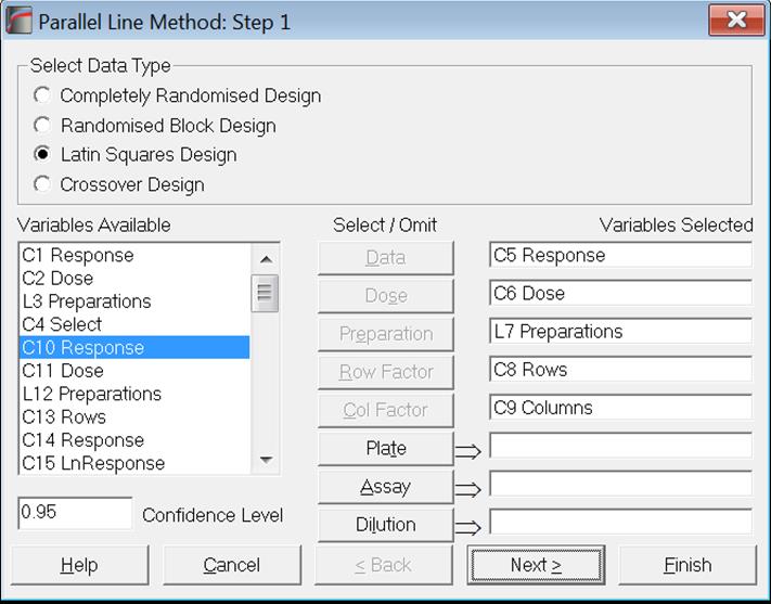
The third and fourth options Latin Square Design and Crossover Design require selection of five variables.
When all variables are selected, click the [Next] button to proceed to Output Options Dialogue.
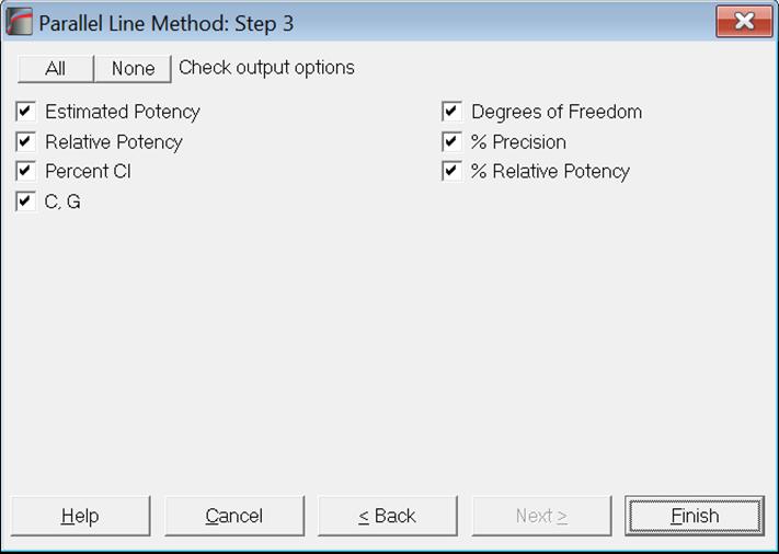
10.1.2. Parallel Line Output Options
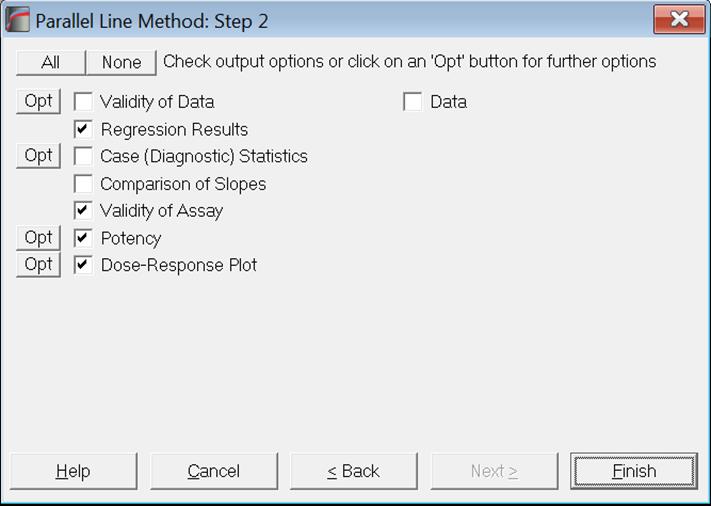
Output options that have further options under them (i.e. further dialogues and windows to display) have an [Opt] button placed to the left of their check boxes. When you click [Finish] without clicking on an [Opt] button first, the program will generate output with default selections. If you want to change the defaults, you can click on the [Opt] button to display further dialogues for this particular output option. Then you can either obtain this particular output option on its own by clicking [Finish], or click [Back] to display the Output Options Dialogue again and output all selected options together.
Data
This output option (which is available for all bioassay analysis methods supported here) will enable the user to include a printout of data used in the analysis as part of the output. This will be useful in fulfilling reporting and data integrity requirements.
Data
|
|
Response |
Dose |
Preparations |
|
1 |
161 |
1 |
Standard S |
|
2 |
151 |
1 |
Preparation T |
|
3 |
162 |
1.5 |
Preparation T |
|
4 |
194 |
2.25 |
Standard S |
|
5 |
176 |
1.5 |
Standard S |
|
6 |
193 |
2.25 |
Preparation T |
|
7 |
160 |
1 |
Preparation T |
|
8 |
192 |
2.25 |
Preparation T |
|
9 |
195 |
2.25 |
Standard S |
|
10 |
184 |
1.5 |
Standard S |
|
11 |
181 |
1.5 |
Preparation T |
|
12 |
166 |
1 |
Standard S |
|
13 |
178 |
1.5 |
Preparation T |
|
14 |
150 |
1 |
Standard S |
|
15 |
174 |
1.5 |
Standard S |
|
16 |
199 |
2.25 |
Preparation T |
|
17 |
201 |
2.25 |
Standard S |
|
18 |
161 |
1 |
Preparation T |
|
19 |
187 |
2.25 |
Standard S |
|
20 |
172 |
1.5 |
Standard S |
|
21 |
161 |
1 |
Standard S |
|
22 |
160 |
1 |
Preparation T |
|
23 |
202 |
2.25 |
Preparation T |
|
24 |
186 |
1.5 |
Preparation T |
|
25 |
171 |
1.5 |
Standard S |
|
26 |
170 |
1.5 |
Preparation T |
|
27 |
193 |
2.25 |
Preparation T |
|
28 |
163 |
1 |
Standard S |
|
29 |
154 |
1 |
Preparation T |
|
30 |
198 |
2.25 |
Standard S |
|
31 |
194 |
2.25 |
Preparation T |
|
32 |
192 |
2.25 |
Standard S |
|
33 |
151 |
1 |
Preparation T |
|
34 |
171 |
1.5 |
Preparation T |
|
35 |
151 |
1 |
Standard S |
|
36 |
182 |
1.5 |
Standard S |
10.1.2.1. Validity of Data
One of the basic assumptions of Parallel Line Method is that for each treatment group (i.e. a unique dose-preparation combination) observations are normally distributed. Normality, homogeneity of variance and outliers of treatment groups can be detected and tested using the following descriptive statistics, tests and plotting procedures provided under this comprehensive menu option.
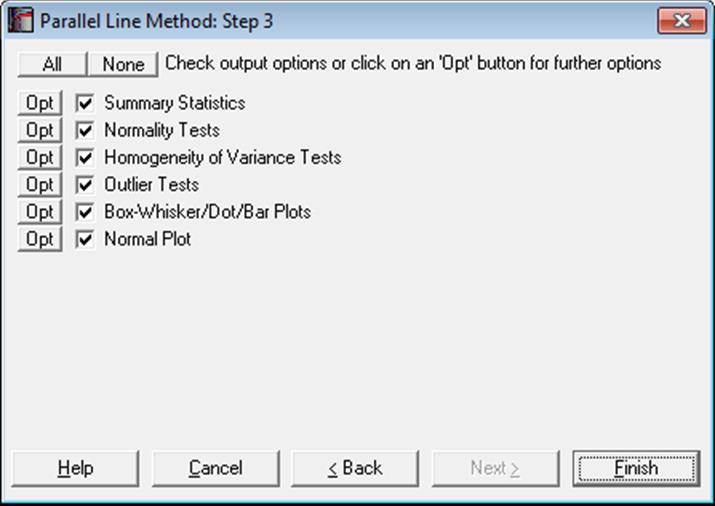
Note that under each test type we provide multiple alternatives. There are four normality tests, five homogeneity of variance tests and three outlier tests. In most cases you will need to use only one of these tests from each type. You can simply uncheck the tests you do not need and UNISTAT will remember your choices in future session.
10.1.2.1.1. Summary Statistics
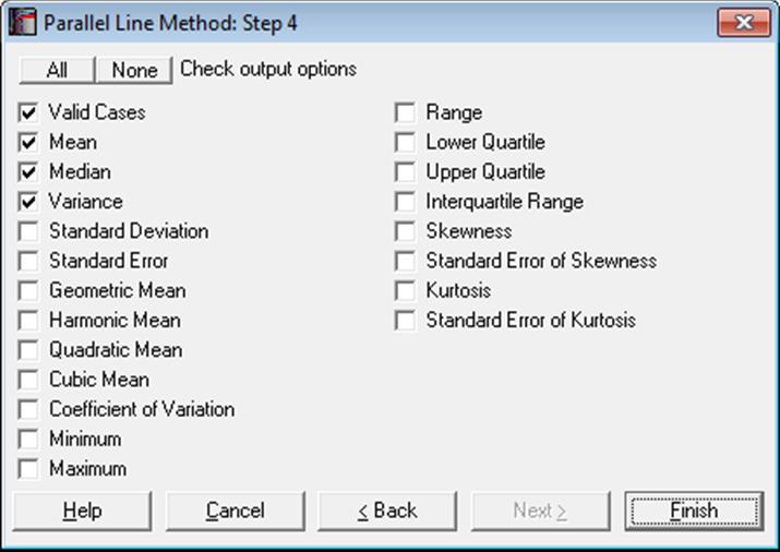
The selected statistics will be displayed for each unique dose-preparation group.
For more information see section 5.1.1. Summary Statistics.
Example
Summary Statistics
Data variable: Response
Subsample selected by: Dose x Preparations
Quantile Method: Simple Average
|
|
Valid Cases |
Mean |
Median |
Variance |
|
1 x Standard S |
6 |
158.6667 |
161.0000 |
43.4667 |
|
1 x Preparation T |
6 |
156.1667 |
157.0000 |
22.1667 |
|
1.5 x Standard S |
6 |
176.5000 |
175.0000 |
28.7000 |
|
1.5 x Preparation T |
6 |
174.6667 |
174.5000 |
75.0667 |
|
2.25 x Standard S |
6 |
194.5000 |
194.5000 |
23.5000 |
|
2.25 x Preparation T |
6 |
195.5000 |
193.5000 |
16.3000 |
10.1.2.1.2. Normality Tests
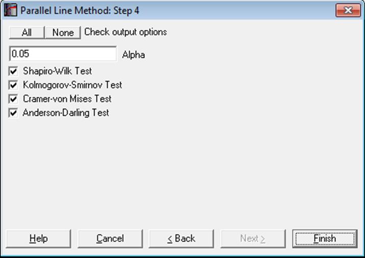
Pass/Fail test results will be displayed by comparing the calculated p-value to the alpha value provided in the above dialogue. Smaller p-values indicate non-normality.
For more information see section 6.3.3. Normality Tests.
Example
Shapiro-Wilk Normality Test
Alpha = 0.05
|
Dose x Preparations |
Test Statistic |
Probability |
Pass/Fail |
|
1 x Standard S |
0.8581 |
0.1827 |
Pass |
|
1 x Preparation T |
0.8118 |
0.0749 |
Pass |
|
1.5 x Standard S |
0.8965 |
0.3536 |
Pass |
|
1.5 x Preparation T |
0.9757 |
0.9284 |
Pass |
|
2.25 x Standard S |
0.9879 |
0.9835 |
Pass |
|
2.25 x Preparation T |
0.8255 |
0.0984 |
Pass |
Kolmogorov-Smirnov Normality Test
Alpha = 0.05
* Lilliefors probability = 0.2 means 0.2 or greater.
|
Dose x Preparations |
Test Statistic |
* Probability |
Pass/Fail |
|
1 x Standard S |
0.3050 |
0.0851 |
Pass |
|
1 x Preparation T |
0.2922 |
0.1177 |
Pass |
|
1.5 x Standard S |
0.2038 |
0.2000 |
Pass |
|
1.5 x Preparation T |
0.1639 |
0.2000 |
Pass |
|
2.25 x Standard S |
0.1364 |
0.2000 |
Pass |
|
2.25 x Preparation T |
0.3115 |
0.0703 |
Pass |
Cramer-von Mises Normality Test
Alpha = 0.05
|
Dose x Preparations |
Test Statistic |
Probability |
Pass/Fail |
|
1 x Standard S |
0.0849 |
0.1450 |
Pass |
|
1 x Preparation T |
0.0886 |
0.1276 |
Pass |
|
1.5 x Standard S |
0.0544 |
0.3902 |
Pass |
|
1.5 x Preparation T |
0.0274 |
0.8514 |
Pass |
|
2.25 x Standard S |
0.0210 |
0.9388 |
Pass |
|
2.25 x Preparation T |
0.1046 |
0.0740 |
Pass |
Anderson-Darling Normality Test
Alpha = 0.05
|
Dose x Preparations |
Test Statistic |
Probability |
Pass/Fail |
|
1 x Standard S |
0.4756 |
0.1438 |
Pass |
|
1 x Preparation T |
0.5470 |
0.0901 |
Pass |
|
1.5 x Standard S |
0.3341 |
0.3689 |
Pass |
|
1.5 x Preparation T |
0.1760 |
0.8637 |
Pass |
|
2.25 x Standard S |
0.1514 |
0.9165 |
Pass |
|
2.25 x Preparation T |
0.5613 |
0.0818 |
Pass |
10.1.2.1.3. Homogeneity of Variance Tests
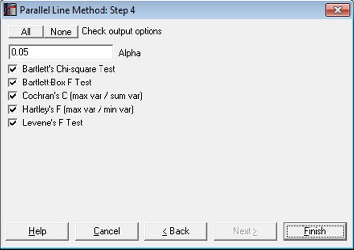
Another basic assumption of Parallel Line Method is that variances for different treatment groups are not significantly different from each other.
Earlier versions of UNISTAT featured Bartlett’s chi-square test as recommended by European Pharmacopoeia (1997-2017), and Hartley’s F test. Here we provide three more homogeneity of variance tests. The computationally demanding Levene’s test is considered to be more powerful than other homogeneity of variance tests.
Test results are displayed as either Pass or Fail, by comparing the calculated p-value to the alpha value provided in the above dialogue. Smaller p-values indicate non-homogeneity.
For a detailed description of these tests see 7.4.2.1. Homogeneity of Variance Test Results.
Example
Homogeneity of Variance Tests
For 6 groups defined by Dose x Preparations.
Alpha = 0.05
|
|
Test Statistic |
Probability |
Pass/Fail |
|
Bartlett’s Chi-square Test |
3.7817 |
0.5813 |
Pass |
|
Bartlett-Box F Test |
0.7637 |
0.5760 |
Pass |
|
Cochran’s C (max var / sum var) |
0.3588 |
0.2313 |
Pass |
|
Hartley’s F (max var / min var) |
4.6053 |
0.0500 |
Pass |
|
Levene’s F Test |
1.5818 |
0.1954 |
Pass |
Hartley’s F probability = 0.05 means 0.05 or greater.
10.1.2.1.4. Outlier Tests
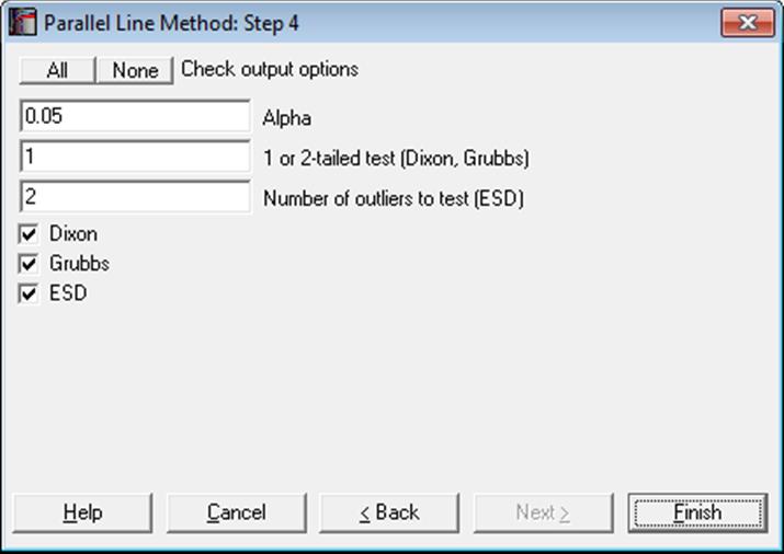
For more information see section 6.3.4. Outlier Tests.
In addition to the tests provided here outliers can also be detected using standardised residuals. See section 10.0.6. Outlier Detection, Omission and Replacement.
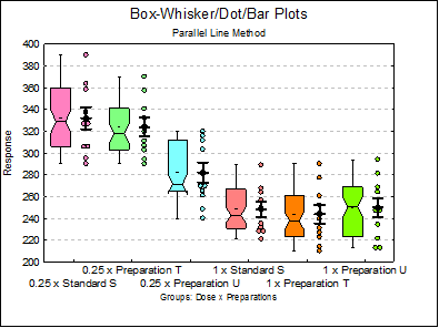
10.1.2.1.5. Box-Whisker, Dot and Bar Plots
This procedure combines boxplot with dot and error bar plots.
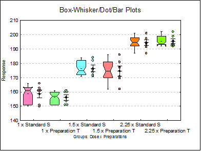
Although all three plot types are displayed on the same graph by default, the user can change graph settings to display any combination of the three plot types, as well as changing other characteristics of the graph. To do this click on the [Opt] button situated to the left of this output option and from the Graphics Editor menu select Edit → Width / Notch / Dots.
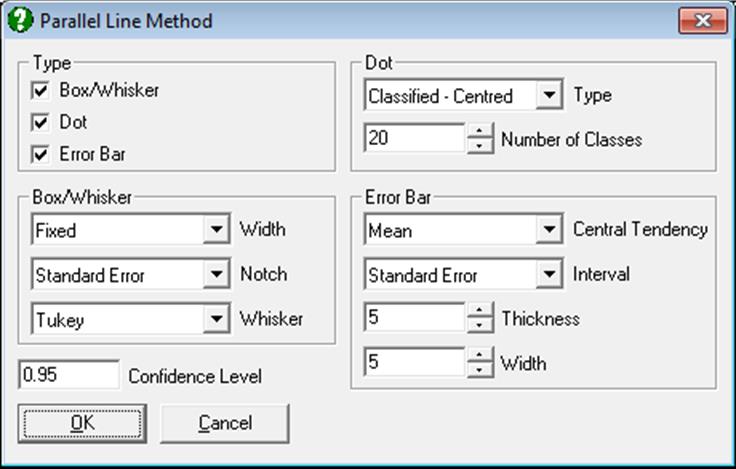
For more information see section 5.3.1. Box-Whisker, Dot and Bar Plots.
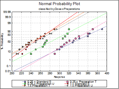
10.1.2.1.6. Normality Plots
By default all treatments are drawn with a line of best fit on a graph with a probit scale Y-axis against the response on a linear X-axis. If the data lies on a near-straight line, then it is said to conform to the normal distribution.
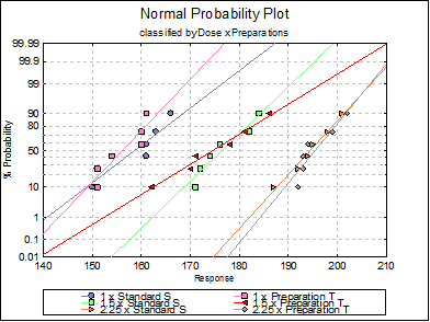
All aspects of the graph can be edited an customised by clicking on the [Opt] button situated to the left of this output option. This will display the Graphics Editor. From the menu select Edit → Data Series.
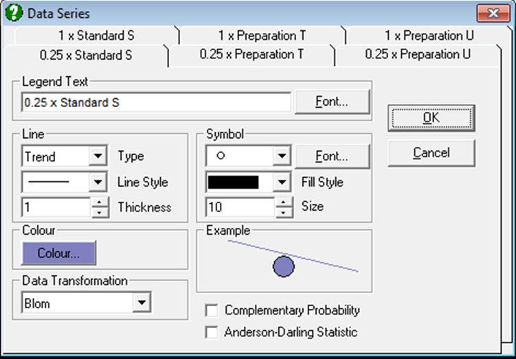
For more information see sections 6.3.3.5. Normality Plots and 5.3.2. Normal Probability Plot.
10.1.2.2. Regression Results
A separate regression line is fitted on each preparation against the natural logarithm of dose. It is also possible to take logs based 10 by entering the following line:
LogBase10=1
C:\ProgramData\Unistat\Unistat10\Unistat10.ini
Example
Separate Regression
|
|
Intercept |
Slope |
Residual SS |
R-squared |
Pass/Fail |
|
Standard S |
248.5800 |
-113.0060 |
1897.7400 |
0.9651 |
Pass |
|
Preparation T |
238.5000 |
-109.5039 |
747.8000 |
0.9851 |
Pass |
Common Regression
|
|
Intercept |
Slope |
Residual SS |
R-squared |
Pass/Fail |
|
Standard S |
247.5150 |
-111.2549 |
2670.7450 |
0.9744 |
Pass |
|
Preparation T |
239.5650 |
|
|
|
|
|
Residual Variance = |
72.1823 |
|
Degrees of Freedom = |
37 |
10.1.2.3. Case (Diagnostic) Statistics
Example
Case (Diagnostic) Statistics
|
|
Response |
Dose |
Preparations |
Estimated Response |
Residuals |
Standardised Residuals |
|
1 |
161 |
1 |
Standard S |
157.7639 |
3.2361 |
0.5684 |
|
2 |
151 |
1 |
Preparation T |
156.6528 |
-5.6528 |
-0.9928 |
|
** 3 |
162 |
1.5 |
Preparation T |
175.4444 |
-13.4444 |
-2.3612 |
|
4 |
194 |
2.25 |
Standard S |
195.3472 |
-1.3472 |
-0.2366 |
|
5 |
176 |
1.5 |
Standard S |
176.5556 |
-0.5556 |
-0.0976 |
|
6 |
193 |
2.25 |
Preparation T |
194.2361 |
-1.2361 |
-0.2171 |
|
7 |
160 |
1 |
Preparation T |
156.6528 |
3.3472 |
0.5879 |
|
8 |
192 |
2.25 |
Preparation T |
194.2361 |
-2.2361 |
-0.3927 |
|
9 |
195 |
2.25 |
Standard S |
195.3472 |
-0.3472 |
-0.0610 |
|
10 |
184 |
1.5 |
Standard S |
176.5556 |
7.4444 |
1.3075 |
|
… |
… |
… |
… |
… |
… |
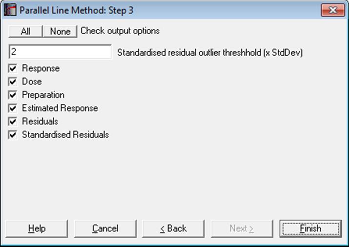
… |
Cases marked by ‘**’ are outliers at 2 x Standard Deviation.
Example
In above example case 3 is reported as an outlier at a two standard deviations threshold. Going back to the spreadsheet, deleting the response value of 162 in row 3 and running the analysis again, we obtain a predicted value of 176.2353 for the omitted outlier.
Case (Diagnostic) Statistics
|
|
Response |
Dose |
Preparations |
Estimated Response |
Residuals |
Standardised Residuals |
|
1 |
161 |
1 |
Standard S |
157.7639 |
3.2361 |
0.6176 |
|
2 |
151 |
1 |
Preparation T |
157.4436 |
-6.4436 |
-1.2298 |
|
* 3 |
* |
1.5 |
Preparation T |
176.2353 |
* |
* |
|
4 |
194 |
2.25 |
Standard S |
195.3472 |
-1.3472 |
-0.2571 |
|
5 |
176 |
1.5 |
Standard S |
176.5556 |
-0.5556 |
-0.1060 |
|
6 |
193 |
2.25 |
Preparation T |
195.0270 |
-2.0270 |
-0.3869 |
|
7 |
160 |
1 |
Preparation T |
157.4436 |
2.5564 |
0.4879 |
|
8 |
192 |
2.25 |
Preparation T |
195.0270 |
-3.0270 |
-0.5777 |
|
9 |
195 |
2.25 |
Standard S |
195.3472 |
-0.3472 |
-0.0663 |
|
10 |
184 |
1.5 |
Standard S |
176.5556 |
7.4444 |
1.4208 |
|
… |
… |
… |
… |
… |
… |
… |
Cases marked by ‘*’ are predicted.
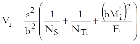
10.1.2.4. Comparison of Slopes
If an assay with two or more test preparations is found to depart from parallelism significantly, then we ask the question which test preparation’s slope differs from the slope of the standard preparation. A Dunnett’s multiple comparison test is performed to answer this question.
Here we perform a Dunnett Test, Comparisons against a Control Group option, using the slope values from Separate Regression. For details see 7.4.3.8. Dunnett test.
The slopes test described in European Pharmacopoeia (1997-2017) employs a slightly different algorithm, which is only valid for 2, 3 or 4-dose assays. It is based on linear contrasts as a proxy for actual slopes. The two approaches are identical and produce the same probability values. UNISTAT does not have a limitation on the number of distinct dose values.
![]()
![]()
L1 is the linear contrast for the standard preparation,
Li is the linear contrast for the ith test preparation and
s2 is the residual mean square value from the ANOVA table (i.e. sum of squares for the overall residual term divided by its degrees of freedom)
The two-tailed probability for the test statistic is generated using an algorithm developed by Charles Dunnett (Algorithm AS 251) for α significance level, (h – 1) number of groups. The degrees of freedom is equal to that of the overall residual term of the ANOVA table.
Example
Comparison of Slopes
|
Comparison |
Difference |
Standard Error |
q Stat |
Table q |
Probability |
|
Preparation T – Standard S |
4.3160 |
5.9453 |
0.7260 |
2.0423 |
0.4735 |
|
Comparison |
Lower 95% |
Upper 95% |
Pass/Fail |
|
Preparation T – Standard S |
-7.8259 |
16.4580 |
Pass |
10.1.2.5. Validity of Assay
This output option displays an Analysis of Variance (ANOVA) table, which is used to test the Validity of Assay. The residual sum of squares and its degrees of freedom are used in estimating the confidence limits for the Potency (see section 10.1.2.6. Potency). The three basic tests performed are (i) significance of regression, (ii) parallelism and (iii) linearity. The table may have different entries in its rows depending on the number of doses and / or the ANOVA model employed.
The notation below is for balanced designs as given by European Pharmacopoeia (1997-2017). For unbalanced designs, the only difference is that the sums are taken up to the maximum number of observations in each treatment group, which can be different. See 10.2. Slope Ratio Method, section 10.2.2.4. Validity of Assay for a general unbalanced formulation.
Let us first define the constant term:
![]()
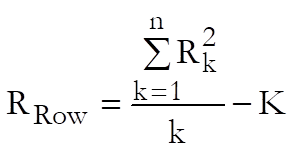
which is the sum total of all cases divided by the total number of treatment groups, the Treatments term:
![]()
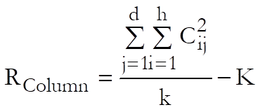
which is the sum of all squared treatment totals minus the constant term, and the Total term:
![]()
which is the sum of all squared cases minus the constant term. The rest of table entries are defined as in the following table. Note that instead of reporting linearity and parallelism, we always report non-linearity and non-parallelism, so that when an F-test gives a significant result (i.e. a low P-value), it means that a data set is not linear or two or more data sets are not parallel. Where possible, we also report non-linearity tests for individual preparations, as well as the overall non-linearity for all preparations.
If you do not wish to display the individual non-linearity values for preparations enter the following line:
NonLinPrepDisp=0
C:\ProgramData\Unistat\Unistat10\Unistat10.ini
QuadraticDisp=0
|
|
Degrees of Freedom |
2-dose |
3-dose |
4-dose |
|
Preparations |
h – 1 |
|
|
|
|
Linear Regression |
1 |
|
|
|
|
Non-parallelism |
h – 1 |
|
|
|
|
Non-linearity |
h for 3-dose 2h for 4-dose |
|
|
|
|
Quadratic Regression |
1 |
|
|
|
|
Difference of Quadratics |
h – 1 |
|
|
|
|
Residual |
h |
|
|
|
|
Treatments |
k – 1 |
M |
M |
M |
|
Residual |
|
R |
R |
R |
|
Total |
nk – 1 |
T |
T |
T |
The following relationships should always be true:
1) Degrees of freedom and sum of squares for the first four rows (i.e. Preparations, Linear Regression, Non-parallelism and Non-linearity) should always add up to Treatments,
2) Quadratic Regression, Difference of Quadratics and their Residuals should always add up to Non-linearity,
3) Treatments (including plate, row and column effects) and their Residuals should always add up to Total.
![]()
![]()
Example
Validity of Assay
|
Due To |
Sum of Squares |
DoF |
Mean Square |
F-Stat |
Prob |
Pass/Fail |
|
Preparations |
11.111 |
1 |
11.111 |
0.535 |
0.4730 |
**Fail** |
|
Linear Regression |
8475.042 |
1 |
8475.042 |
408.108 |
0.0000 |
Pass |
|
Non-parallelism |
18.375 |
1 |
18.375 |
0.885 |
0.3581 |
Pass |
|
Non-linearity |
5.472 |
2 |
2.736 |
0.132 |
0.8773 |
Pass |
|
Standard S Non-linearity |
0.028 |
1 |
0.028 |
0.001 |
0.9712 |
Pass |
|
Preparation T Non-linearity |
5.444 |
1 |
5.444 |
0.262 |
0.6142 |
Pass |
|
Quadratic Regression |
3.125 |
1 |
3.125 |
0.150 |
0.7022 |
|
|
Quadratic Difference |
2.347 |
1 |
2.347 |
0.113 |
0.7402 |
|
|
Treatments |
8510.000 |
5 |
1702.000 |
81.958 |
0.0000 |
Pass |
|
Blocks(Rows) |
412.000 |
5 |
82.400 |
3.968 |
0.0116 |
|
|
Blocks(Columns) |
218.667 |
5 |
43.733 |
2.106 |
0.1069 |
|
|
Residual |
415.333 |
20 |
20.767 |
|
|
|
|
Total |
9556.000 |
35 |
273.029 |
|
|
|
10.1.2.6. Potency
By default, the program estimates the potency ratio and its confidence limits employing the generalised algorithm given in Finney (1978), which works with unbalanced, symmetric and balanced designs. European Pharmacopoeia (1997-2017) gives a more restrictive algorithm for balanced assays only. The logarithm of potency ratio is estimated for each test preparation, using the Common Regression slope b.
![]()
and:
![]()
where:
![]()
are the preparation means and Ai is the assumed potency of each test preparation. The estimated potency is the antilog of M, Exp(M).
The method of estimating the confidence interval for potency is based on Fieller’s Theorem (see Finney 1978, p. 80). Let us first define the correction factor g as:
![]()
where E is the sum of squares for the Linear
Regression term and s2 is the residual mean squares from the
ANOVA table. ![]() is the critical value from
the t-distribution with the same degrees of freedom. The confidence limits computed
below are reliable for g < 1. If this condition is not fulfilled, the
program will issue a warning message, but still display the confidence limits
computed.
is the critical value from
the t-distribution with the same degrees of freedom. The confidence limits computed
below are reliable for g < 1. If this condition is not fulfilled, the
program will issue a warning message, but still display the confidence limits
computed.
The log of confidence limits for the potency ratio of each test preparation is defined as:
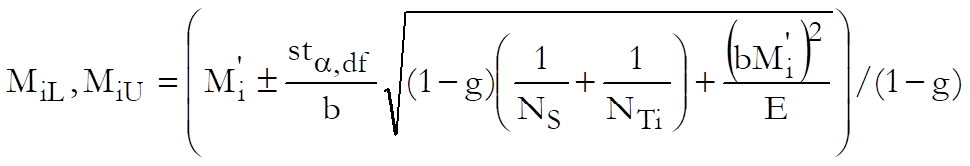
where the variance of Mi is:
Weights are computed after the estimated potency and its confidence interval are found:
![]()
and % Precision is:
![]()
According to European Pharmacopoeia (1997) the common slope b is calculated as:
![]()
![]()
Where:
Z = Log(dosei+1) – Log(dosei), i = 2, … , d
is the log of successive dose ratios. Also define a correction factor:
![]()
where E is the sum of squares for the Linear
Regression term and s2 is the residual mean squares and ![]() is the critical value from the
t-distribution with degrees of freedom of the overall residual term from the
ANOVA table.
is the critical value from the
t-distribution with degrees of freedom of the overall residual term from the
ANOVA table.
The log of the corrected potency estimate and its confidence intervals are computed as:
![]()
where:
![]()
The only difference from the default output here is reporting of C and H constants for validation purposes, where C = 1 / (1 – g).
If the data column [Dose] contains the actual dose levels administered in original dose units, we will obtain the estimated potency and its confidence limits in the same units. If, however, the [Dose] column contains unitless relative dose levels, then we may need to perform further calculations to obtain the estimated potency in original units. To do that you can enter assigned potency of the standard, assumed potency of each test preparation and pre-dilutions for all preparations including the standard in a data column and select it as [Dilution] variable. UNISTAT will then calculate the estimated potency as described in section 10.0.2. Doses, Dilutions and Potency. Also see section 10.0.3. Potency Calculation Example.
Example
Potency
Latin Squares Design
|
|
Estimated Potency |
Lower 95% |
Upper 95% |
DoF |
% Precision |
|
Preparation T |
0.9763 |
0.9112 |
1.0456 |
20 |
93.33% |
|
|
Relative Potency |
Lower 95% |
Upper 95% |
|
Preparation T |
97.63% |
91.12% |
104.56% |
|
|
Percent CI |
Lower 95% |
Upper 95% |
Pass/Fail |
|
Preparation T |
100.00% |
93.33% |
107.09% |
Pass |
PotencyPctLower: 93.3289382317094 GT 75 Pass
AND
PotencyPctUpper: 107.0925498258 LT 125 Pass
|
G = |
0.0107 |
|
C = |
1.0108 |
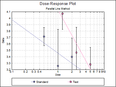
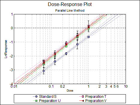
10.1.2.7. Dose-Response Plot
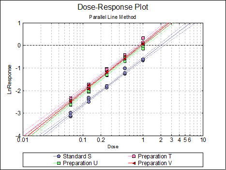
By default, this option generates a plot of treatment means against the log of dose, with standard error bars for each mean. Each preparation will be plotted as one data series, with as many points as the number of doses applied. A line of best fit and its confidence limits will be drawn for each series. This provides a visual means of inspecting the data, enabling the user to notice immediately whether there is something substantially wrong with the data.
Alternatively, individual response values can be plotted against the log of dose, all with or without trend lines and confidence intervals.
Clicking the [Opt] button situated to the left of Dose-Response Plot output option will place the graph in UNISTAT’s Graphics Editor. Here, all aspects of the graph can be edited and customised.
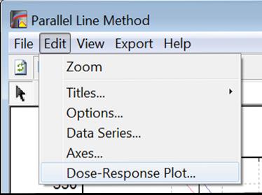
Selecting Edit → Dose-Response Plot… (or double-clicking on the graph area) will pop a dialogue where what is displayed on the plot can be controlled.
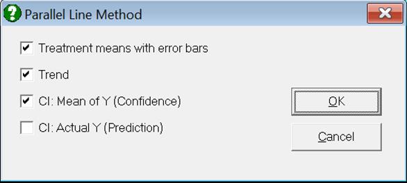
If you uncheck the Treatment means with error bars box, individual response values will be plotted against the log of dose.
10.1.3. Parallel Line Examples
The following Parallel Line Method examples are based on different Analysis of Variance methods. Data sets were entered into UNISTAT’s spreadsheet and necessary data manipulations made by using UNISTAT spreadsheet functions (see 10.0.1. Data Preparation and 10.0.2. Doses, Dilutions and Potency). Final data sets were saved in two files; BIOPHARMA9 which contains examples from European Pharmacopoeia (2017, the 9th Edition) and BIOFINNEY containing examples from Finney (1978).
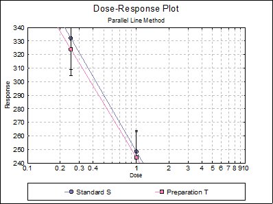
10.1.3.1. Completely Randomised Design with 2 Doses and 3 Preparations
Data is given in Table 5.1.1-I. on p. 4364 of European Pharmacopoeia (9th Edition).
Open BIOPHARMA9 and select Bioassay → Parallel Line Method. From the Variable Selection Dialogue select the first option Completely Randomised Design and then select columns C1, C2 and L3 respectively as [Data], [Dose] and [Preparation]. Click [Next] to proceed to Output Options Dialogue. Click [All] to perform all tests in one go and click [Finish]. The following output is obtained:
Parallel Line Method
Valid Number of Cases: 60, 0 Omitted
Completely Randomised Design
Summary Statistics
Data variable: Response
Subsample selected by: Dose x Preparations
|
|
Valid Cases |
Mean |
Variance |
Standard Error |
|
0.25 x Standard S |
10 |
332.0000 |
1026.6667 |
10.1325 |
|
0.25 x Preparation T |
10 |
323.9000 |
724.9889 |
8.5146 |
|
0.25 x Preparation U |
10 |
282.2000 |
854.6222 |
9.2446 |
|
1 x Standard S |
10 |
248.4000 |
483.8222 |
6.9557 |
|
1 x Preparation T |
10 |
244.0000 |
718.6667 |
8.4774 |
|
1 x Preparation U |
10 |
250.0000 |
784.6667 |
8.8581 |
Anderson-Darling Normality Test
Alpha = 0.05
|
Dose x Preparations |
Test Statistic |
Probability |
Pass/Fail |
|
0.25 x Standard S |
0.2218 |
0.7658 |
Pass |
|
0.25 x Preparation T |
0.2311 |
0.7326 |
Pass |
|
0.25 x Preparation U |
0.5030 |
0.1549 |
Pass |
|
1 x Standard S |
0.3494 |
0.3962 |
Pass |
|
1 x Preparation T |
0.2337 |
0.7232 |
Pass |
|
1 x Preparation U |
0.2055 |
0.8201 |
Pass |
Homogeneity of Variance Tests
For 6 groups defined by Dose x Preparations.
Alpha = 0.05
|
|
Test Statistic |
Probability |
Pass/Fail |
|
Levene’s F Test |
0.3738 |
0.8644 |
Pass |
Dixon’s Outlier Test
Alpha = 0.05
One-tailed tests
|
Dose x Preparations |
Dixon’s Q |
Table Q |
Pass/Fail |
|
0.25 x Standard S Q(Min) |
0.1351 |
0.4779 |
Pass |
|
Q(Max) |
0.2889 |
0.4779 |
Pass |
|
0.25 x Preparation T Q(Min) |
0.0714 |
0.4779 |
Pass |
|
Q(Max) |
0.1333 |
0.4779 |
Pass |
|
0.25 x Preparation U Q(Min) |
0.1299 |
0.4779 |
Pass |
|
Q(Max) |
0.0429 |
0.4779 |
Pass |
|
1 x Standard S Q(Min) |
0.1667 |
0.4779 |
Pass |
|
Q(Max) |
0.3333 |
0.4779 |
Pass |
|
1 x Preparation T Q(Min) |
0.0857 |
0.4779 |
Pass |
|
Q(Max) |
0.1351 |
0.4779 |
Pass |
|
1 x Preparation U Q(Min) |
0.0429 |
0.4779 |
Pass |
|
Q(Max) |
0.1410 |
0.4779 |
Pass |
N = 10, Q(Min)=(X(2)-X(1))/(X(N-1)-X(1)), Q(Max)=(X(N)-X(N-1))/(X(N)-X(2))
Separate Regression
|
|
Intercept |
Slope |
Residual SS |
R-squared |
|
Standard S |
248.4000 |
-60.3047 |
13594.4000 |
0.7199 |
|
Preparation T |
244.0000 |
-57.6357 |
12992.9000 |
0.7107 |
|
Preparation U |
250.0000 |
-23.2274 |
14753.6000 |
0.2600 |
Common Regression
|
|
Intercept |
Slope |
Residual SS |
R-squared |
|
Standard S |
257.5833 |
-47.0559 |
49559.1333 |
0.5629 |
|
Preparation T |
251.3333 |
|
|
|
|
Preparation U |
233.4833 |
|
|
|
|
Residual Variance = |
884.9845 |
|
Degrees of Freedom = |
56 |
Case (Diagnostic) Statistics
|
|
Response |
Dose |
Preparations |
Estimated Response |
Residuals |
Standardised Residuals |
|
1 |
300 |
0.25 |
Standard S |
322.8167 |
-22.8167 |
-0.7670 |
|
2 |
310 |
0.25 |
Standard S |
322.8167 |
-12.8167 |
-0.4308 |
|
3 |
330 |
0.25 |
Standard S |
322.8167 |
7.1833 |
0.2415 |
|
4 |
290 |
0.25 |
Standard S |
322.8167 |
-32.8167 |
-1.1031 |
|
5 |
364 |
0.25 |
Standard S |
322.8167 |
41.1833 |
1.3844 |
|
6 |
328 |
0.25 |
Standard S |
322.8167 |
5.1833 |
0.1742 |
|
** 7 |
390 |
0.25 |
Standard S |
322.8167 |
67.1833 |
2.2584 |
|
8 |
360 |
0.25 |
Standard S |
322.8167 |
37.1833 |
1.2499 |
|
9 |
342 |
0.25 |
Standard S |
322.8167 |
19.1833 |
0.6448 |
|
10 |
306 |
0.25 |
Standard S |
322.8167 |
-16.8167 |
-0.5653 |
|
11 |
289 |
1 |
Standard S |
257.5833 |
31.4167 |
1.0561 |
|
12 |
221 |
1 |
Standard S |
257.5833 |
-36.5833 |
-1.2297 |
|
13 |
267 |
1 |
Standard S |
257.5833 |
9.4167 |
0.3165 |
|
… |
… |
… |
… |
… |
… |
… |
Cases marked by ‘**’ are outliers at 2 x Standard Deviation.
Comparison of Slopes
|
Comparison |
Difference |
Standard Error |
q Stat |
Table q |
|
Preparation U – Standard S |
37.0773 |
12.6231 |
2.9372 |
2.2713 |
|
Preparation T – Standard S |
2.6690 |
12.6231 |
0.2114 |
2.2713 |
|
Comparison |
Probability |
Lower 95% |
Upper 95% |
Result |
|
Preparation U – Standard S |
0.0093 |
8.4061 |
65.7484 |
**Fail** |
|
Preparation T – Standard S |
0.9678 |
-26.0022 |
31.3401 |
Pass |
Validity of Assay
|
Due To |
Sum of Squares |
DoF |
Mean Square |
F-Stat |
Prob |
|
Preparations |
6256.633 |
2 |
3128.317 |
4.086 |
0.0223 |
|
Linear Regression |
63830.817 |
1 |
63830.817 |
83.377 |
0.0000 |
|
Non-parallelism |
8218.233 |
2 |
4109.117 |
5.367 |
0.0075 |
|
Non-linearity |
0.000 |
0 |
|
|
|
|
Treatments |
78305.683 |
5 |
15661.137 |
20.457 |
0.0000 |
|
Residual |
41340.900 |
54 |
765.572 |
|
|
|
Total |
119646.583 |
59 |
2027.908 |
|
|
Potency
|
|
Estimated Potency |
Lower 95% |
Upper 95% |
DoF |
% Precision |
|
Preparation T |
1.1420 |
0.7836 |
1.6869 |
54 |
68.62% |
|
Preparation U |
1.6689 |
1.1481 |
2.5550 |
54 |
68.80% |
|
|
Relative Potency |
Lower 95% |
Upper 95% |
|
Preparation T |
114.20% |
78.36% |
168.69% |
|
Preparation U |
166.89% |
114.81% |
255.50% |
|
|
Percent CI |
Lower 95% |
Upper 95% |
|
Preparation T |
100.00% |
68.62% |
147.71% |
|
Preparation U |
100.00% |
68.80% |
153.10% |
|
G = |
0.0482 |
|
C = |
1.0507 |
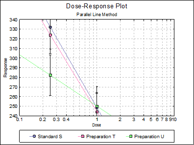
Looking at the plot of treatment means we can see that Preparation U line is not nearly parallel to Standard S and Preparation T lines. This can also be picked up from the non-parallelism test in Validity of Assay (0.0075), which is significant at 5% level. The Comparison of Slopes test also reports a significant difference between Preparation U and Standard S slopes.
This assay can still be useful by omitting Preparation U and performing the analysis for Standard S and Preparation U. In Excel Add-In Mode, you can simply select the block A1:C41 and repeat the analysis. In Stand-Alone Mode, you can define a Select Row column to omit these rows from the analysis, without actually deleting them from the spreadsheet. To do this, click somewhere on column 4, and select Data → Select Row option from UNISTAT’s spreadsheet menus. The colour of C4 will change. This indicates that all rows with a 0 entry in this column will be omitted from the subsequent analyses.
When the analysis is repeated without Preparation U, the following results are obtained:
Parallel Line Method
Rows 41-60 Omitted
Selected by C4 Select
Valid Number of Cases: 40, 20 Omitted
Completely Randomised Design
Separate Regression
|
|
Intercept |
Slope |
Residual SS |
R-squared |
|
Standard S |
248.4000 |
-60.3047 |
13594.4000 |
0.7199 |
|
Preparation T |
244.0000 |
-57.6357 |
12992.9000 |
0.7107 |
Common Regression
|
|
Intercept |
Slope |
Residual SS |
R-squared |
|
Standard S |
249.3250 |
-58.9702 |
26621.5250 |
0.7151 |
|
Preparation T |
243.0750 |
|
|
|
|
Residual Variance = |
719.5007 |
|
Degrees of Freedom = |
37 |
Comparison of Slopes
|
Comparison |
Difference |
Standard Error |
q Stat |
Table q |
|
Preparation T – Standard S |
2.6690 |
12.3983 |
0.2153 |
2.0281 |
|
Comparison |
Probability |
Lower 95% |
Upper 95% |
Result |
|
Preparation T – Standard S |
0.8308 |
-22.4759 |
27.8138 |
Pass |
Validity of Assay
|
Due To |
Sum of Squares |
DoF |
Mean Square |
F-Stat |
Prob |
|
Preparations |
390.625 |
1 |
390.625 |
0.529 |
0.4718 |
|
Linear Regression |
66830.625 |
1 |
66830.625 |
90.491 |
0.0000 |
|
Non-parallelism |
34.225 |
1 |
34.225 |
0.046 |
0.8308 |
|
Non-linearity |
0.000 |
0 |
|
|
|
|
Treatments |
67255.475 |
3 |
22418.492 |
30.355 |
0.0000 |
|
Residual |
26587.300 |
36 |
738.536 |
|
|
|
Total |
93842.775 |
39 |
2406.225 |
|
|
Potency
|
|
Estimated Potency |
Lower 95% |
Upper 95% |
DoF |
% Precision |
|
Preparation T |
1.1118 |
0.8250 |
1.5136 |
36 |
74.20% |
|
|
Relative Potency |
Lower 95% |
Upper 95% |
|
Preparation T |
111.18% |
82.50% |
151.36% |
|
|
Percent CI |
Lower 95% |
Upper 95% |
|
Preparation T |
100.00% |
74.20% |
136.14% |
|
G = |
0.0455 |
|
C = |
1.0476 |
In Stand-Alone Mode, do not forget to reset column 4, otherwise the Select Row function will be effective in subsequent procedures you run. To do this, click somewhere on column 4, and select Data → Select Row option again, or select Formula → Quick Formula from the menu and enter data. The colour of C4 will change back to its original state.
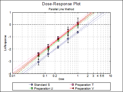
10.1.3.2. Completely Randomised Design with 5 Doses and 4 Preparations
Data is given in Table 5.1.4-I. on p. 4367 of European Pharmacopoeia (9th Edition).
Open BIOPHARMA9 and select Bioassay → Parallel Line Method. From the Variable Selection Dialogue select the first option Completely Randomised Design and then select columns C17, C18, L19 and L20 respectively as [Data], [Dose], [Preparation] and [Dilution]. Click [Next] to proceed to Output Options Dialogue, select only the following output options and click [Finish]:
Parallel Line Method
Valid Number of Cases: 60, 0 Omitted
Completely Randomised Design
Separate Regression
|
|
Intercept |
Slope |
Residual SS |
R-squared |
|
Standard S |
-0.5998 |
0.8813 |
0.0904 |
0.9920 |
|
Preparation T |
0.1355 |
0.9037 |
0.1208 |
0.9898 |
|
Preparation U |
-0.0226 |
0.9278 |
0.0843 |
0.9933 |
|
Preparation V |
0.0714 |
0.9211 |
0.0459 |
0.9963 |
Common Regression
|
|
Intercept |
Slope |
Residual SS |
R-squared |
|
Standard S |
-0.5621 |
0.9085 |
0.3600 |
0.9925 |
|
Preparation T |
0.1422 |
|
|
|
|
Preparation U |
-0.0495 |
|
|
|
|
Preparation V |
0.0539 |
|
|
|
|
Residual Variance = |
0.0065 |
|
Degrees of Freedom = |
55 |
Comparison of Slopes
|
Comparison |
Difference |
Standard Error |
q Stat |
Table q |
|
Preparation U – Standard S |
0.0466 |
0.0304 |
1.5296 |
2.4415 |
|
Preparation V – Standard S |
0.0398 |
0.0304 |
1.3074 |
2.4415 |
|
Preparation T – Standard S |
0.0224 |
0.0304 |
0.7365 |
2.4415 |
|
Comparison |
Probability |
Lower 95% |
Upper 95% |
Result |
|
Preparation U – Standard S |
0.3036 |
-0.0278 |
0.1209 |
Pass |
|
Preparation V – Standard S |
0.4262 |
-0.0345 |
0.1141 |
Pass |
|
Preparation T – Standard S |
0.8033 |
-0.0519 |
0.0967 |
Pass |
Validity of Assay
|
Due To |
Sum of Squares |
DoF |
Mean Square |
F-Stat |
Prob |
|
Preparations |
4.475 |
3 |
1.492 |
223.395 |
0.0000 |
|
Linear Regression |
47.584 |
1 |
47.584 |
7125.912 |
0.0000 |
|
Non-parallelism |
0.019 |
3 |
0.006 |
0.933 |
0.4339 |
|
Non-linearity |
0.074 |
12 |
0.006 |
0.926 |
0.5307 |
|
Standard S Non-linearity |
0.017 |
3 |
0.006 |
0.850 |
0.4747 |
|
Preparation T Non-linearity |
0.028 |
3 |
0.009 |
1.410 |
0.2538 |
|
Preparation U Non-linearity |
0.018 |
3 |
0.006 |
0.886 |
0.4564 |
|
Preparation V Non-linearity |
0.011 |
3 |
0.004 |
0.559 |
0.6455 |
|
Treatments |
52.152 |
19 |
2.745 |
411.053 |
0.0000 |
|
Residual |
0.267 |
40 |
0.007 |
|
|
|
Total |
52.419 |
59 |
0.888 |
|
|
Potency
Assumed potency of Preparation T: 20 µg protein/ml
Assumed potency of Preparation U: 20 µg protein/ml
Assumed potency of Preparation V: 20 µg protein/ml
|
|
Estimated Potency |
Lower 95% |
Upper 95% |
|
Preparation T |
43.4197 |
40.5448 |
46.5397 |
|
Preparation U |
35.1628 |
32.8697 |
37.6403 |
|
Preparation V |
39.4018 |
36.8126 |
42.2058 |
|
|
Relative Potency |
Lower 95% |
Upper 95% |
|
Preparation T |
217.10% |
202.72% |
232.70% |
|
Preparation U |
175.81% |
164.35% |
188.20% |
|
Preparation V |
197.01% |
184.06% |
211.03% |
|
|
Percent CI |
Lower 95% |
Upper 95% |
|
Preparation T |
100.00% |
93.38% |
107.19% |
|
Preparation U |
100.00% |
93.48% |
107.05% |
|
Preparation V |
100.00% |
93.43% |
107.12% |
|
G = |
0.0006 |
|
C = |
1.0006 |
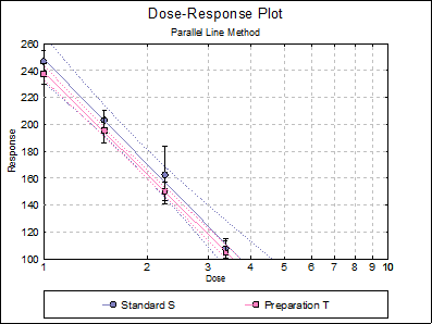
10.1.3.3. Randomised Block Design with 4 Doses and 2 Preparations
Data is given in Table 5.1.3.-I on p. 4366 of European Pharmacopoeia (9th Edition).
Open BIOPHARMA9 and select Bioassay → Parallel Line Method. From the Variable Selection Dialogue select the second option Randomised Block Design and the select columns C11, C12, L13, C14 and L15 respectively as [Data], [Dose], [Preparation], [Row Factor] and [Dilution]. Click [Next] to proceed to the Output Options Dialogue.
Parallel Line Method
Valid Number of Cases: 40, 0 Omitted
Randomised Block Design
Separate Regression
|
|
Intercept |
Slope |
Residual SS |
R-squared |
|
Standard S |
248.5800 |
-113.0060 |
1897.7400 |
0.9651 |
|
Preparation T |
238.5000 |
-109.5039 |
747.8000 |
0.9851 |
Common Regression
|
|
Intercept |
Slope |
Residual SS |
R-squared |
|
Standard S |
247.5150 |
-111.2549 |
2670.7450 |
0.9744 |
|
Preparation T |
239.5650 |
|
|
|
Comparison of Slopes
|
Comparison |
Difference |
Standard Error |
q Stat |
Table q |
|
Preparation T – Standard S |
3.5022 |
5.1221 |
0.6837 |
2.0484 |
|
Comparison |
Probability |
Lower 95% |
Upper 95% |
Result |
|
Preparation T – Standard S |
0.4998 |
-6.9901 |
13.9944 |
Pass |
Validity of Assay
|
Due To |
Sum of Squares |
DoF |
Mean Square |
F-Stat |
Prob |
|
Preparations |
632.025 |
1 |
632.025 |
11.722 |
0.0019 |
|
Linear Regression |
101745.605 |
1 |
101745.605 |
1887.111 |
0.0000 |
|
Non-parallelism |
25.205 |
1 |
25.205 |
0.467 |
0.4998 |
|
Non-linearity |
259.140 |
4 |
64.785 |
1.202 |
0.3321 |
|
Standard S Non-linearity |
238.140 |
2 |
119.070 |
2.208 |
0.1287 |
|
Preparation T Non-linearity |
21.000 |
2 |
10.500 |
0.195 |
0.8241 |
|
Quadratic Regression |
148.225 |
1 |
148.225 |
2.749 |
0.1085 |
|
Quadratic Difference |
34.225 |
1 |
34.225 |
0.635 |
0.4323 |
|
Residual |
76.690 |
2 |
38.345 |
|
|
|
Treatments |
102661.975 |
7 |
14665.996 |
272.015 |
0.0000 |
|
Blocks(Rows) |
876.750 |
4 |
219.188 |
4.065 |
0.0101 |
|
Residual |
1509.650 |
28 |
53.916 |
|
|
|
Total |
105048.375 |
39 |
2693.548 |
|
|
Potency
Randomised Block Design
Assigned potency of Standard S: 670 IU/mg
Pre-dilution of Standard S: 16.7 mg / 25 ml; 1 ml / 40 ml
Assumed potency of Preparation T: 20000 IU/vial
Pre-dilution of Preparation T: 1 vial / 40 ml; 1 ml / 40 ml
|
|
Estimated Potency |
Lower 95% |
Upper 95% |
|
Preparation T |
19228.4755 |
18423.3508 |
20075.1776 |
|
|
Relative Potency |
Lower 95% |
Upper 95% |
|
Preparation T |
107.41% |
102.91% |
112.14% |
|
|
Percent CI |
Lower 95% |
Upper 95% |
|
Preparation T |
100.00% |
95.81% |
104.40% |
|
G = |
0.0022 |
|
C = |
1.0022 |
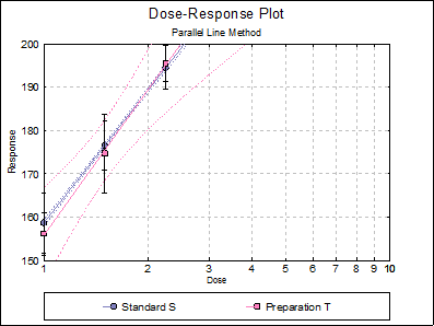
10.1.3.4. Latin Square Design with 3 Doses and 2 Preparations
Data is given in Table 5.1.2.-II on p. 4367 of European Pharmacopoeia (9th Edition).
The entry and transformation of this data set is more complicated than the two previous examples. In order to assign the correct dose levels and preparation groups, information given in Table 5.1.2.-I is essential. Ensure that the way the factor columns are created is understood well.
Open BIOPHARMA9 and select Bioassay → Parallel Line Method. From the Variable Selection Dialogue select the third option Latin Square Design and then select columns C5, C6, L7, C8, C9 and L10 respectively as [Data], [Dose], [Preparation], [Row Factor], [Col Factor] and [Dilution]. Click [Next] to proceed to Output Options Dialogue.
Parallel Line Method
Valid Number of Cases: 36, 0 Omitted
Latin Squares Design
Separate Regression
|
|
Intercept |
Slope |
Residual SS |
R-squared |
|
Standard S |
158.6389 |
44.1879 |
478.3611 |
0.8895 |
|
Preparation T |
155.7778 |
48.5040 |
573.1111 |
0.8901 |
Common Regression
|
|
Intercept |
Slope |
Residual SS |
R-squared |
|
Standard S |
157.7639 |
46.3460 |
1069.8472 |
0.8879 |
|
Preparation T |
156.6528 |
|
|
|
|
Residual Variance = |
32.4196 |
|
Degrees of Freedom = |
33 |
Comparison of Slopes
|
Comparison |
Difference |
Standard Error |
q Stat |
Table q |
|
Preparation T – Standard S |
4.3160 |
4.5883 |
0.9407 |
2.0860 |
|
Comparison |
Probability |
Lower 95% |
Upper 95% |
Result |
|
Preparation T – Standard S |
0.3581 |
-5.2551 |
13.8871 |
Pass |
Validity of Assay
|
Due To |
Sum of Squares |
DoF |
Mean Square |
F-Stat |
Prob |
|
Preparations |
11.111 |
1 |
11.111 |
0.535 |
0.4730 |
|
Linear Regression |
8475.042 |
1 |
8475.042 |
408.108 |
0.0000 |
|
Non-parallelism |
18.375 |
1 |
18.375 |
0.885 |
0.3581 |
|
Non-linearity |
5.472 |
2 |
2.736 |
0.132 |
0.8773 |
|
Standard S Non-linearity |
0.028 |
1 |
0.028 |
0.001 |
0.9712 |
|
Preparation T Non-linearity |
5.444 |
1 |
5.444 |
0.262 |
0.6142 |
|
Quadratic Regression |
3.125 |
1 |
3.125 |
0.150 |
0.7022 |
|
Quadratic Difference |
2.347 |
1 |
2.347 |
0.113 |
0.7402 |
|
Treatments |
8510.000 |
5 |
1702.000 |
81.958 |
0.0000 |
|
Blocks(Rows) |
412.000 |
5 |
82.400 |
3.968 |
0.0116 |
|
Blocks(Columns) |
218.667 |
5 |
43.733 |
2.106 |
0.1069 |
|
Residual |
415.333 |
20 |
20.767 |
|
|
|
Total |
9556.000 |
35 |
273.029 |
|
|
Potency
Latin Squares Design
Assigned potency of Standard S: 4855 IU/mg
Pre-dilution of Standard S: 25.2 mg / 24.5 ml
Assumed potency of Preparation T: 5600 IU/mg
Pre-dilution of Preparation T: 21.4 mg / 23.95 ml
|
|
Estimated Potency |
Lower 95% |
Upper 95% |
|
Preparation T |
5456.3665 |
5092.3689 |
5843.3620 |
|
|
Relative Potency |
Lower 95% |
Upper 95% |
|
Preparation T |
97.63% |
91.12% |
104.56% |
|
|
Percent CI |
Lower 95% |
Upper 95% |
|
Preparation T |
100.00% |
93.33% |
107.09% |
|
G = |
0.0107 |
|
C = |
1.0108 |
10.1.3.5. Twin Crossover Design
Data is given in Table 5.1.5-II. on p. 4368 of European Pharmacopoeia (9th Edition).
Open BIOPHARMA9 and select Bioassay → Parallel Line Method. From the Variable Selection Dialogue select the fourth option Crossover Design and select columns C21, C22, L23, C24, C25 and L26 respectively as [Data], [Dose], [Preparation], [Row Factor] and [Col Factor]. Click [Next] to proceed to Output Options Dialogue and then click [Finish]. The following output is obtained:
Parallel Line Method
Valid Number of Cases: 64, 0 Omitted
Crossover Design
Separate Regression
|
|
Intercept |
Slope |
Residual SS |
R-squared |
|
Standard |
101.1875 |
-47.6991 |
19294.1875 |
0.3119 |
|
Test |
91.5625 |
-20.1977 |
23815.8750 |
0.0618 |
Common Regression
|
|
Intercept |
Slope |
Residual SS |
R-squared |
|
Standard |
96.4219 |
-33.9484 |
44563.5781 |
0.1658 |
|
Test |
96.3281 |
|
|
|
|
Residual Variance = |
730.5505 |
|
Degrees of Freedom = |
61 |
Comparison of Slopes
|
Comparison |
Difference |
Standard Error |
q Stat |
Table q |
|
Test – Standard |
27.5014 |
8.4520 |
3.2538 |
2.0484 |
|
Comparison |
Probability |
Lower 95% |
Upper 95% |
Result |
|
Test – Standard |
0.0030 |
10.1882 |
44.8146 |
**Fail** |
Validity of Assay
|
Due To |
Sum of Squares |
DoF |
Mean Square |
F-Stat |
Prob |
|
Non-parallelism |
1453.5156 |
1 |
1453.5156 |
1.0638 |
0.3112 |
|
DaysxPreparations |
31.6406 |
1 |
31.6406 |
0.0232 |
0.8801 |
|
DaysxLinear Regression |
50.7656 |
1 |
50.7656 |
0.0372 |
0.8485 |
|
Error Between |
38258.8125 |
28 |
1366.3862 |
|
|
|
Blocks(Rows) |
39794.7344 |
31 |
1283.7011 |
|
|
|
Preparations |
0.1406 |
1 |
0.1406 |
0.0010 |
0.9747 |
|
Linear Regression |
8859.5156 |
1 |
8859.5156 |
64.5324 |
0.0000 |
|
Days |
478.5156 |
1 |
478.5156 |
3.4855 |
0.0724 |
|
DaysxNon-parallelism |
446.2656 |
1 |
446.2656 |
3.2506 |
0.0822 |
|
Error Within |
3844.0625 |
28 |
137.2879 |
|
|
|
Total |
53423.2344 |
63 |
847.9878 |
|
|
Potency
Crossover Design
Assumed potency of Test: 40 IU/ml
|
|
Estimated Potency |
Lower 95% |
Upper 95% |
|
Test |
40.1106 |
33.4162 |
48.1646 |
|
|
Relative Potency |
Lower 95% |
Upper 95% |
|
Test |
100.28% |
83.54% |
120.41% |
|
|
Percent CI |
Lower 95% |
Upper 95% |
|
Test |
100.00% |
83.31% |
120.08% |
|
G = |
0.0650 |
|
C = |
1.0695 |
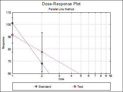
Although the plot of treatment means and the Comparison of Slopes test seem to indicate deviation from parallelism, the non-parallelism test in Validity of Assay (0.3112) is not significant at 5% level.
10.1.3.6. Triple Crossover Design
Table 10.3.1. on p. 205 from Finney, D. J. (1978) is an example with three dose levels and two preparations.
Open BIOFINNEY and select Bioassay → Parallel Line Method. From the Variable Selection Dialogue select the fourth option Crossover Design and select columns C15, C16, S17, C18 and C19 respectively as [Data], [Dose], [Preparation], [Row Factor] and [Col Factor]. Click [Next] to proceed to Output Options Dialogue and click [Finish].
Parallel Line Method
Valid Number of Cases: 60, 0 Omitted
Crossover Design
Separate Regression
|
|
Intercept |
Slope |
Residual SS |
R-squared |
|
Standard |
3.4547 |
-0.2272 |
8.1200 |
0.0576 |
|
Test |
4.1272 |
-0.5713 |
5.2830 |
0.3725 |
Common Regression
|
|
Intercept |
Slope |
Residual SS |
R-squared |
|
Standard |
3.4547 |
-0.3993 |
13.9718 |
0.1798 |
|
Test |
3.9695 |
|
|
|
|
Residual Variance = |
0.2451 |
|
Degrees of Freedom = |
57 |
Comparison of Slopes
|
Comparison |
Difference |
Standard Error |
q Stat |
Table q |
|
Test – Standard |
-0.3441 |
0.1209 |
2.8455 |
2.0639 |
|
Comparison |
Probability |
Lower 95% |
Upper 95% |
Result |
|
Test – Standard |
0.0089 |
-0.5937 |
-0.0945 |
**Fail** |
Validity of Assay
|
Due To |
Sum of Squares |
DoF |
Mean Square |
F-Stat |
Prob |
|
Non-parallelism |
0.5688 |
1 |
0.5688 |
1.6032 |
0.2176 |
|
Quadratic Regression |
0.8687 |
1 |
0.8687 |
2.4484 |
0.1307 |
|
DaysxPreparations |
0.3481 |
1 |
0.3481 |
0.9810 |
0.3318 |
|
DaysxLinear Regression |
0.0031 |
1 |
0.0031 |
0.0086 |
0.9267 |
|
DaysxQuadratic Difference |
1.9026 |
1 |
1.9026 |
5.3624 |
0.0294 |
|
Error Between |
8.5153 |
24 |
0.3548 |
|
|
|
Blocks(Rows) |
12.2066 |
29 |
0.4209 |
|
|
|
Preparations |
0.3330 |
1 |
0.3330 |
4.7403 |
0.0395 |
|
Linear Regression |
3.0636 |
1 |
3.0636 |
43.6087 |
0.0000 |
|
Days |
0.0150 |
1 |
0.0150 |
0.2141 |
0.6477 |
|
Quadratic Difference |
0.0261 |
1 |
0.0261 |
0.3716 |
0.5478 |
|
DaysxNon-parallelism |
0.0164 |
1 |
0.0164 |
0.2335 |
0.6333 |
|
DaysxQuadratic Regression |
0.0216 |
1 |
0.0216 |
0.3075 |
0.5844 |
|
Error Within |
1.6861 |
24 |
0.0703 |
|
|
|
Total |
17.3685 |
59 |
0.2944 |
|
|
Potency
|
|
Estimated Potency |
Lower 95% |
Upper 95% |
|
Test |
0.2754 |
0.1783 |
0.3923 |
|
G = |
0.0977 |
|
C = |
1.1083 |