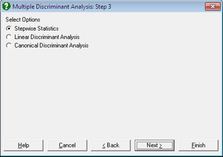
8.2.1. Multiple Discriminant Analysis
Linear and Canonical discriminant analyses can be performed with or without stepwise selection of variables. A Linear Discriminant Analysis should be performed before a Canonical one. The program will do this automatically, even if only the Canonical option is selected. It is possible to output Stepwise Statistics, Linear and Canonical analysis results separately.
8.2.1.1. Stepwise Discriminant Analysis
The Stepwise check box provided on the Variable Selection Dialogue enables you to select the best subset of variables to run a Discriminant Analysis. When this box is checked, the variables selected for analysis are ranked according to their influence on the final result. They are also tested against a user-defined criterion of eligibility. The variable with the highest influence that passes the test of eligibility is then included in the analysis. At each step, the already selected variables are also tested against an exclusion criterion and they may be excluded from the analysis if they fail to satisfy this criterion. The steps are repeated until there are no variables that can be entered or removed from the analysis.
The stepwise selection method used in Stepwise Discriminant Analysis is almost identical to the one employed in Stepwise Regression. For further information on this method and the interpretation of F-to-enter and F-to-remove statistics see 7.2.3.1. Stepwise Selection Criteria. The following output options are available:
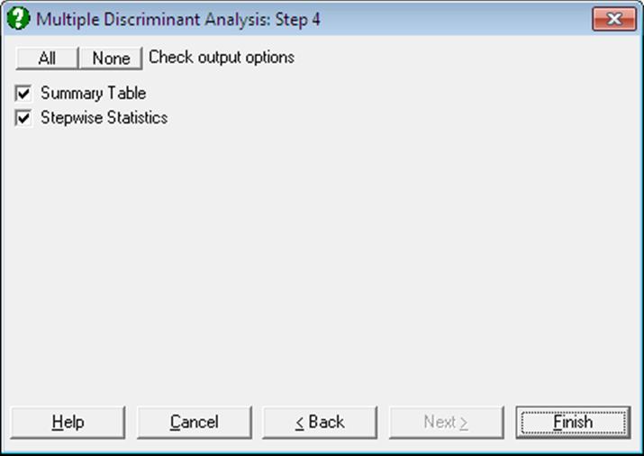
Summary Table: The variable entered or removed at each step, its F-to-enter or F-to-remove value, its tail probability and Wilks’ lambda statistic are displayed.
Stepwise Statistics: First, within group sums of squares and the cross product matrix are computed:
![]()
where g is the number of groups, p is the number of
variables, xijk is the value
of variable i for case k in group j and mj is the number of cases in group j. Define ![]() as the new matrix after a new variable
is entered or omitted. Then:
as the new matrix after a new variable
is entered or omitted. Then:
Tolerancei = 0 if ![]()
Tolerancei = ![]() if
variable i is not in the analysis,
if
variable i is not in the analysis,
Tolerancei = ![]() if
variable i is in the analysis.
if
variable i is in the analysis.
![]()
with degrees of freedom (g – 1) and (n – p – g + 1),
![]()
with degrees of freedom (g – 1) and (n – p – g),
and Wilks’ Lambda is:
![]()
8.2.1.2. Linear Discriminant Analysis
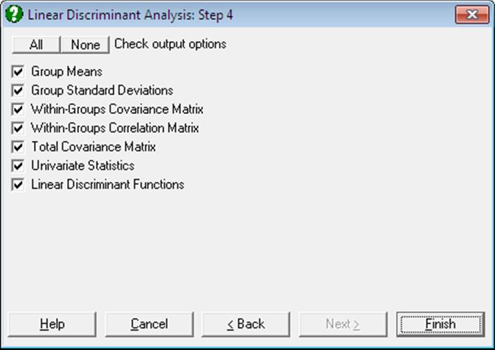
Group Means and Standard Deviations: The means and standard deviations of sub-groups defined by the factor column are tabulated.
Pooled Within-Groups Covariance Matrix:
[wil/(n-g)]
Pooled Within-Groups Correlation Matrix:
[wil/Sqr(wiiwll)].
Total Covariance Matrix: First compute the total sums of squares and cross product matrix:
![]()
The total covariance matrix is [til/(n – 1)].
Univariate Statistics: Wilks’ lambda is:
![]()
and the F-statistic, which has g – 1 and n – g degrees of freedom, is:
![]()
Linear Discriminant Functions: These are also known as Fisher’s Linear Discriminant Functions. The coefficients can be saved to the data matrix and subsequently used to classify cases. Since canonical discrimination is a superior method, classifications are made here in the second level Output Options Dialogue, using the Canonical Discrimination Functions.
Coefficients of the Linear Discriminant Functions are:
![]()
where i = 1, …, p and j = 1, …, g and the constant terms are:
![]()
where pj = nj/n.
8.2.1.3. Canonical Discriminant Analysis
The Canonical Discriminant Analysis is based on the eigenvectors and eigenvalues of the proximity matrix and thus it involves an iterational algorithm. Iterations continue until either the reduction in the objective function is less than a given tolerance level, or the maximum number of iterations is reached.
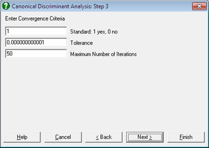
A dialogue allows editing two or three parameters, depending on whether the data is raw or it is already formed into a proximity matrix (i.e. it is square and symmetric). In the former case, the program will allow the choice of forming a standardised (the default) or non standardised proximity matrix.
The eigenvalues and eigenvectors of the system are found using the Cholesky decomposition.
The number of Canonical Discriminant Functions extracted (f) depends on the number of variables and the number of groups:
f = Min(p, g – 1)
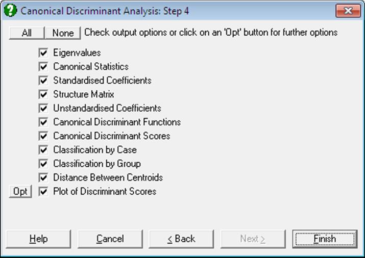
where p is the number of variables and g is the number of groups. The output options include the following:
Eigenvalues: Canonical Correlations are found as:
![]()
Canonical Statistics: Wilks’ lambda is used to test the significance of all the discriminating functions after the first k:
![]()
The tail probability for lambda is determined from chi-square distribution:
![]()
with (p – k)(g – k – 1) degrees of freedom.
Canonical Discriminant Coefficients: Standardised coefficients matrix D is obtained by multiplying the square roots of [wii] by the corresponding eigenvectors. The unstandardised coefficients are:
![]()
and the constants are:
![]()
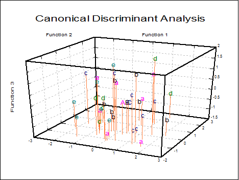
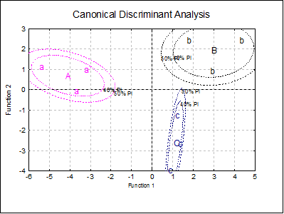
Canonical Discriminant Scores: The unstandardised coefficients matrix is multiplied by the data matrix. Discriminant scores can be displayed in tabular form and saved to the Data Processor for further analysis. They can also be displayed in 2D and 3D scatter diagrams with group memberships and group centroids. Centroids are the Canonical Discriminant Functions evaluated at the group means.
![]()
Classification by Case: For each case, the chi-square distances from all centroids are computed. The probability of the case being a member of a group is the tail probability for this chi-square value with m degrees of freedom. A case is classified into the group for which this probability is the highest.
The table displays the given group membership, the highest probability (estimated) group, and the probability of the case belonging to the estimated group. If the estimated and actual groups differ, two stars (representing a misclassification) are printed between the two columns.
Classification by Group: This is an alternative way of presenting the classification results explained above. A table is formed with rows and columns corresponding to actual and estimated group memberships respectively. Each cell displays the number of elements and their percentage. Diagonal elements are the cases classified correctly and the off-diagonal elements are misclassified cases.
Distance Between Centroids: The distance between every pair of centroids are tabulated in ascending order.
Plot of Discriminant Scores: This provides options to display group centroids (which are represented by capital letters) and groups selectively. If you select two variables a 2D graph is displayed and a 3D graph if you select three variables.
You can choose to display group centroids in capital letters, point labels or change the font of group letters from the Edit → XY Points dialogue. When the Cluster No field is zero all groups will be displayed simultaneously. If this field is set to one, then the first group only, if two, the second group only, etc., will be displayed.
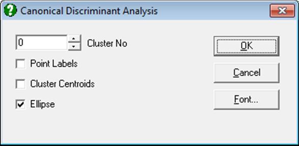
For 2D plots, by checking the Ellipse box on, you can draw interval curves for the mean of Y (confidence) and / or actual Y (prediction) values at one or more confidence levels. For further details see Ellipse Confidence and Prediction Intervals in 4.1.1.1.1. Line.
8.2.1.4. Discriminant Examples
Example 1
Table 11.1 on p. 513 from Tabachnick, B. G. & L. S. Fidell (1989). Measurements on four predictors, performance, information, verbal expression and age, are given on three groups of children. In order to keep track of group memberships of children we should add a factor column Group to the data matrix. We would like to find out whether the children have been correctly classified into three groups. We would also like to be able to determine the group membership of a child who was not included in the study, but for whom we have measurements on predictor variables.
Open MULTIVAR, select Statistics 2 → Discriminant Analysis → Multiple Discriminant Analysis and select Perf, Info, Verbexp, Age (C1 to C4) as [Variable]s and Group (C5) as [Factor]. Leave the Stepwise box unchecked. The analysis has two stages; first a Linear Discriminant Analysis is performed and its output options are presented alongside the option for the second stage; Canonical Discriminant Analysis. Select all output options in both stages to obtain the following results:
Linear Discriminant Analysis
Group Means
|
|
Perf |
Info |
Verbexp |
Age |
|
Group 1 |
98.6667 |
7.0000 |
36.3333 |
7.3000 |
|
Group 2 |
87.6667 |
11.6667 |
38.3333 |
6.9333 |
|
Group 3 |
101.3333 |
9.6667 |
28.3333 |
7.6333 |
Group Standard Deviations
|
|
Perf |
Info |
Verbexp |
Age |
|
Group 1 |
12.5831 |
2.0000 |
5.5076 |
0.9539 |
|
Group 2 |
13.2035 |
3.7859 |
6.5064 |
0.7024 |
|
Group 3 |
17.6163 |
2.0817 |
1.5275 |
1.1590 |
Within-Groups Covariance Matrix
|
|
Perf |
Info |
Verbexp |
Age |
|
Perf |
214.3333 |
36.6667 |
58.0556 |
8.3333 |
|
Info |
36.6667 |
7.5556 |
12.2778 |
1.0611 |
|
Verbexp |
58.0556 |
12.2778 |
25.0000 |
1.6222 |
|
Age |
8.3333 |
1.0611 |
1.6222 |
0.9156 |
Within-Groups Correlation Matrix
|
|
Perf |
Info |
Verbexp |
Age |
|
Perf |
1.0000 |
0.9112 |
0.7931 |
0.5949 |
|
Info |
0.9112 |
1.0000 |
0.8933 |
0.4034 |
|
Verbexp |
0.7931 |
0.8933 |
1.0000 |
0.3391 |
|
Age |
0.5949 |
0.4034 |
0.3391 |
1.0000 |
Total Covariance Matrix
|
|
Perf |
Info |
Verbexp |
Age |
|
Perf |
200.1111 |
18.5556 |
21.0417 |
8.0611 |
|
Info |
18.5556 |
9.7778 |
10.2083 |
0.5181 |
|
Verbexp |
21.0417 |
10.2083 |
39.7500 |
-0.0833 |
|
Age |
8.0611 |
0.5181 |
-0.0833 |
0.7786 |
Univariate Statistics
|
|
Lambda |
F-statistic |
Probability |
|
Perf |
0.8033 |
0.7346 |
0.5184 |
|
Info |
0.5795 |
2.1765 |
0.1947 |
|
Verbexp |
0.4717 |
3.3600 |
0.1050 |
|
Age |
0.8819 |
0.4017 |
0.6859 |
Linear Discriminant Functions
|
|
Group 1 |
Group 2 |
Group 3 |
|
Perf |
1.9242 |
0.5870 |
1.3655 |
|
Info |
-17.5622 |
-8.6992 |
-10.5870 |
|
Verbexp |
5.5459 |
4.1168 |
2.9728 |
|
Age |
0.9872 |
5.0175 |
2.9114 |
|
Constant |
-138.9111 |
-72.3844 |
-72.3403 |
Canonical Discriminant Analysis
Eigenvalues
|
|
Eigenvalue |
Percent |
Cumulative |
Correlation |
|
1 |
13.4859 |
70.7% |
70.7% |
0.9649 |
|
2 |
5.5892 |
29.3% |
100.0% |
0.9210 |
Canonical Statistics
|
|
Wilks’ lambda |
Chi-square |
Deg Fre |
Probability |
|
0 |
0.0105 |
20.5138 |
8 |
0.0086 |
|
1 |
0.1518 |
8.4845 |
3 |
0.0370 |
Standardised Coefficients
|
|
Function 1 |
Function 2 |
|
Perf |
-2.5035 |
-1.4741 |
|
Info |
3.4896 |
-0.2838 |
|
Verbexp |
-1.3247 |
1.7888 |
|
Age |
0.5027 |
0.2362 |
Structure Matrix
|
|
Function 1 |
Function 2 |
|
Perf |
-0.0755 |
-0.1734 |
|
Info |
0.2280 |
0.0664 |
|
Verbexp |
-0.0223 |
0.4463 |
|
Age |
-0.0279 |
-0.1486 |
Unstandardised Coefficients
|
|
Function 1 |
Function 2 |
|
Perf |
-0.1710 |
-0.1007 |
|
Info |
1.2695 |
-0.1032 |
|
Verbexp |
-0.2649 |
0.3578 |
|
Age |
0.5254 |
0.2469 |
|
Constant |
9.6737 |
-3.4529 |
Canonical Discriminant Functions
|
|
Function 1 |
Function 2 |
|
Group 1 |
-4.1023 |
0.6910 |
|
Group 2 |
2.9807 |
1.9417 |
|
Group 3 |
1.1217 |
-2.6327 |
Canonical Discriminant Scores
|
|
Function 1 |
Function 2 |
|
1 |
-3.7063 |
-0.0581 |
|
2 |
-3.2036 |
0.9864 |
|
3 |
-5.3972 |
1.1446 |
|
4 |
4.2997 |
2.4526 |
|
5 |
1.7594 |
2.4276 |
|
6 |
2.8829 |
0.9448 |
|
7 |
0.8531 |
-3.9675 |
|
8 |
1.1866 |
-1.2645 |
|
9 |
1.3253 |
-2.6660 |
Classification by Case
|
|
ActGroup |
EstGroup |
Probability |
|
1 |
1 |
1 |
0.6984 |
|
2 |
1 |
1 |
0.6392 |
|
3 |
1 |
1 |
0.3902 |
|
4 |
2 |
2 |
0.3677 |
|
5 |
2 |
2 |
0.4215 |
|
6 |
2 |
2 |
0.6055 |
|
7 |
3 |
3 |
0.3958 |
|
8 |
3 |
3 |
0.3914 |
|
9 |
3 |
3 |
0.9789 |
Classification by Group
|
|
Group 1 |
Group 2 |
Group 3 |
|
Group 1 |
3 |
0 |
0 |
|
Group 2 |
0 |
3 |
0 |
|
Group 3 |
0 |
0 |
3 |
Correctly classified: 100.00%
Distance Between Centroids
|
Clusters |
Distance |
|
B – C |
4.9377 |
|
A – C |
6.1917 |
|
A – B |
7.1926 |
Example 2
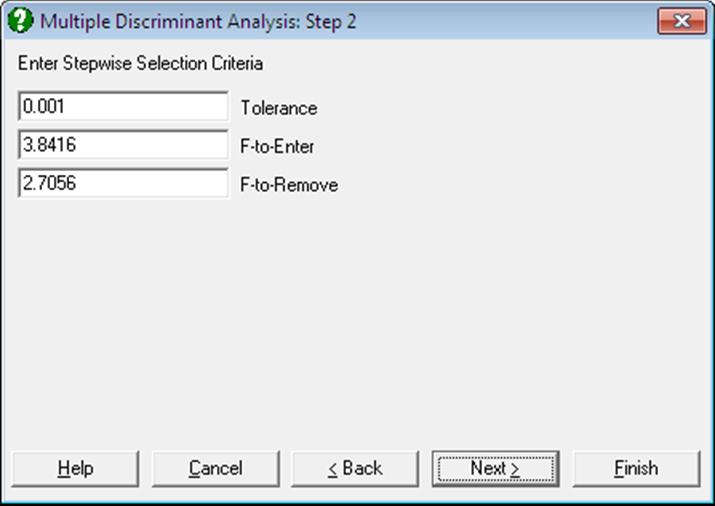
Open STEPDSCR, select Statistics 2 → Discriminant Analysis → Multiple Discriminant Analysis and select Var1, to Var7 (C1 to C7) as [Variable]s, Groups (C8) as [Factor] and check the Stepwise box. On the next dialogue, accept the default values of Tolerance, F-to-Enter and F-to-Remove. Next select Stepwise Statistics and leave both output options checked. The output below is abbreviated:
Multiple Discriminant Analysis: Stepwise Statistics
Summary Table
Tolerance: 0.001
F-to-Enter: 3.8416 (5.0%)
F-to-Remove: 2.7056 (10.0%)
|
Variable |
Entered at Step |
F-to-Enter |
Probability |
Wilks’ Lambda |
|
Var3 |
1 |
42.2648 |
0.0000 |
0.6167 |
|
Var5 |
2 |
9.1029 |
0.0036 |
0.5429 |
|
Var7 |
3 |
7.7673 |
0.0070 |
0.4858 |
|
Var6 |
4 |
10.7627 |
0.0017 |
0.4168 |
Step 0
|
Variable |
Entered at Step |
Tolerance |
F-to-Enter/Remove |
Wilks’ Lambda |
|
Var1 |
|
1.0000 |
4.0471 |
0.9438 |
|
Var2 |
|
1.0000 |
0.7221 |
0.9895 |
|
Var3 |
|
1.0000 |
42.2648 |
0.6167 |
|
Var4 |
|
1.0000 |
0.1175 |
0.9983 |
|
Var5 |
|
1.0000 |
24.2906 |
0.7368 |
|
Var6 |
|
1.0000 |
0.1060 |
0.9984 |
|
Var7 |
|
1.0000 |
2.0781 |
0.9703 |
…
Step 4
|
Variable |
Entered at Step |
Tolerance |
F-to-Enter/Remove |
Wilks’ Lambda |
|
Var1 |
|
0.9923 |
0.8803 |
0.4111 |
|
Var2 |
|
0.9777 |
3.1368 |
0.3973 |
|
Var3 |
1 |
-1.0000 |
35.3364 |
0.6433 |
|
Var4 |
|
0.9910 |
2.3970 |
0.4017 |
|
Var5 |
2 |
-1.0000 |
7.9404 |
0.4677 |
|
Var6 |
4 |
-1.0000 |
10.7627 |
0.4858 |
|
Var7 |
3 |
-1.0000 |
19.3810 |
0.5410 |