5.1.4. Sample Statistics
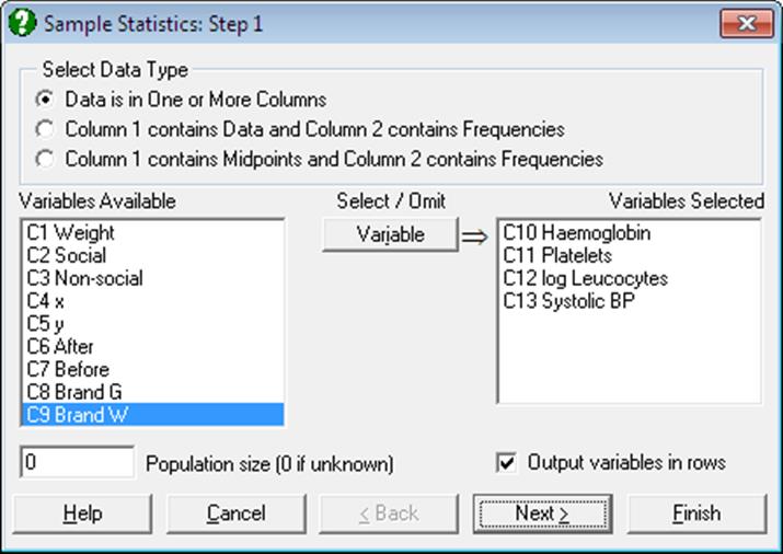
The Variable Selection Dialogue for this procedure offers three types of data to analyse (see 5.0.2. One-Sample Data Types). A text box is also provided on this dialogue to enter the size of the total population from which the sample is drawn. The default value of 0 means that the total population is not known and the program assumes an infinite population. A non-zero population value affects only the standard error of mean in output.
The Output variables in rows check box allows you to transpose the output matrix. This will be useful when you wish to use the output from this procedure (such as means and standard errors) for further analysis in other procedures.
Output for different data options differ slightly. For instance, the grouped data output includes the Sheppard’s correction for the second and fourth moments but it does not include minimum, maximum and range.
For ungrouped data, the method used in computing the median, lower and upper quartiles is indicated in the output. This can be one of the six methods described in the previous section 5.1.3.1. Quantile Methods.
The following statistics can be calculated for ungrouped (option 1) and frequency and grouped data (options 2 and 3). Let n be the number of valid observations (i.e. excluding missing values) and fi the frequency of data point Xi given in column 2. Note that for ungrouped data fi = 1, i = 1, …, n.
Size: Number of cases (rows) in the sample, including missing values.
Missing: Number of missing cases in the sample. In frequency and grouped data a case is considered missing when either or both of value and frequency are missing.
Total Frequency:
![]()
N = n for ungrouped data.
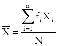
Mean: The weighted arithmetic mean is:
Geometric Mean: The weighted geometric mean is:
![]()
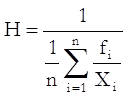
Harmonic Mean: The weighted harmonic mean is:
The following relationship should hold if Xi ≥ 0, i = 1, …, n:
![]()
Median: For ungrouped data, this is computed using the quantile method selected in step two of the Quantiles (Percentiles) procedure, as described in section 5.1.3.1. Quantile Methods.
For frequency and grouped data, both value and frequency columns are sorted in ascending order according to values. For frequency data, half of total frequency is found and the median is calculated as above. For grouped data, median is calculated by interpolation as:
where:
· L is the lower class boundary of the class containing the median,
· the summation term is the sum of frequencies of all classes lower than the median class,
· C is the size of median class interval and
· N is the total frequency as defined above.
Lower Quartile: Calculations are similar to that of median, except for 25% quantile instead of 50%.
Upper Quartile: Calculations are similar to that of median, except for 75% quantile instead of 50%.
Interquartile Range: Difference between upper and lower quartiles.
Minimum: Smallest observed value in data (not available for grouped data).
Maximum: Greatest observed value in data (not available for grouped data).
Range: Difference between maximum and minimum values (not available for grouped data).
Sum: The weighted sum is:
![]()
Sum of Squares: The weighted sum of squares is:
![]()
Root Mean Square (Quadratic mean):
![]()
Unbiased Variance:
Unbiased Standard Deviation:
![]()
Standard Error of Mean:
![]()
Standard Error with Finite Population Correction: Available only when total population is known and it is greater than the total frequency.
![]()
Coefficient of Variation:
![]()
Variance:
![]()
Standard Deviation:
![]()
Sheppard’s Correction for 2nd Moment (Variance): Available for only grouped data:
![]()
where C is the size of uniform class interval.
Mean Deviation:
3rd Moment About the Mean:
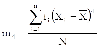
4th Moment About the Mean:
Unbiased 3rd Moment:
![]()
Sheppard’s Correction for the 4th Moment: Available for only grouped data:
![]()
where C is the size of uniform class interval.
Moment Coefficient of Skewness:
![]()
An alternative definition of skewness is given in section 5.1.1. Summary Statistics.
Moment Coefficient of Kurtosis:
![]()
An alternative definition of kurtosis is given in section 5.1.1. Summary Statistics.
Pearson’s Second Coefficient of Skewness:
![]()
Example 1: Ungrouped data
Open PARTEST and select Statistics 1 → Descriptive Statistics → Sample Statistics. Select Haemoglobin, Platelets, log Leucocytes, and Systolic BP (C10 to C13) as [Variable]s, uncheck the Output variables in rows box and click [Finish].
Sample Statistics
Quantile Method: Simple Average
|
|
Haemoglobin |
Platelets |
log Leucocytes |
Systolic BP |
|
Size |
10.0000 |
10.0000 |
10.0000 |
10.0000 |
|
Missing |
0.0000 |
0.0000 |
0.0000 |
0.0000 |
|
Mean |
-0.5300 |
-0.0300 |
-0.5900 |
3.1000 |
|
Geometric Mean |
* |
* |
* |
* |
|
Harmonic Mean |
* |
* |
* |
* |
|
Median |
-0.6000 |
0.1000 |
-0.6500 |
2.0000 |
|
Lower Quartile |
-1.5000 |
-1.0000 |
-1.6000 |
-2.0000 |
|
Upper Quartile |
0.0000 |
0.6000 |
0.9000 |
8.0000 |
|
Interquartile Range |
1.5000 |
1.6000 |
2.5000 |
10.0000 |
|
Minimum |
-2.4000 |
-2.2000 |
-3.2000 |
-6.0000 |
|
Maximum |
2.3000 |
1.9000 |
1.7000 |
14.0000 |
|
Range |
4.7000 |
4.1000 |
4.9000 |
20.0000 |
|
Sum |
-5.3000 |
-0.3000 |
-5.9000 |
31.0000 |
|
Sum of Squares |
22.0700 |
13.3900 |
25.1700 |
437.0000 |
|
Root Mean Square |
1.4856 |
1.1572 |
1.5865 |
6.6106 |
|
Unbiased Variance |
2.1401 |
1.4868 |
2.4099 |
37.8778 |
|
Unbiased Standard Deviation |
1.4629 |
1.2193 |
1.5524 |
6.1545 |
|
Standard Error of Mean |
0.4626 |
0.3856 |
0.4909 |
1.9462 |
|
Coefficient of Variation |
-2.6186 |
-38.5588 |
-2.4961 |
1.8834 |
|
Variance |
1.9261 |
1.3381 |
2.1689 |
34.0900 |
|
Standard Deviation |
1.3878 |
1.1568 |
1.4727 |
5.8387 |
|
Mean Deviation |
1.1500 |
0.9020 |
1.2500 |
4.9200 |
|
3rd Moment About Mean |
1.3179 |
-0.4318 |
-0.1544 |
69.6720 |
|
4th Moment About Mean |
9.2971 |
4.2938 |
9.5652 |
2527.7857 |
|
Unbiased 3rd Moment |
1.8304 |
-0.5998 |
-0.2144 |
96.7667 |
|
Moment Coefficient of Skewness |
0.4930 |
-0.2790 |
-0.0483 |
0.3500 |
|
Moment Coefficient of Kurtosis |
2.5060 |
2.3981 |
2.0334 |
2.1751 |
|
Pearson’s Skewness Coefficient |
0.1513 |
-0.3371 |
0.1222 |
0.5652 |
Example 2: Variables in rows
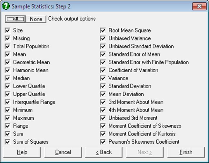
Continuing from the last example, go back to Variable Selection Dialogue, check the Output variables in rows box and click [Next]. From the Output Options Dialogue select only the last three options and click [Finish].
Sample Statistics
|
|
Moment Coefficient of Skewness |
Moment Coefficient of Kurtosis |
Pearson’s Skewness Coefficient |
|
Haemoglobin |
0.4930 |
2.5060 |
0.1513 |
|
Platelets |
-0.2790 |
2.3981 |
-0.3371 |
|
log Leucocytes |
-0.0483 |
2.0334 |
0.1222 |
|
Systolic BP |
0.3500 |
2.1751 |
0.5652 |
Example 3: Frequency data
Open TIMESER, select Statistics 1 → Descriptive Statistics → Sample Statistics and select the second data option Column 1 contains Data and Column 2 contains Frequencies. Select Surface Area (C13) as [Column 1] and Blemishes (C14) as [Column 2] and enter 150 in the Total Population box. The following results are obtained:
Sample Statistics
Surface Area: contains data, Blemishes contains frequencies
|
|
Surface Area |
|
Size |
20.0000 |
|
Missing |
0.0000 |
|
Total Frequency |
94.0000 |
|
Total Population |
150.0000 |
|
Mean |
0.8462 |
|
Geometric Mean |
0.8265 |
|
Harmonic Mean |
0.8070 |
|
… |
… |
|
Root Mean Square |
0.8653 |
|
Unbiased Variance |
0.0330 |
|
Unbiased Standard Deviation |
0.1817 |
|
Standard Error of Mean |
0.0187 |
|
Standard Error with Finite Population |
0.0115 |
|
Coefficient of Variation |
0.2136 |
|
Variance |
0.0327 |
|
Standard Deviation |
0.1807 |
|
Mean Deviation |
0.1443 |
|
3rd Moment About Mean |
0.0004 |
|
4th Moment About Mean |
0.0017 |
|
Unbiased 3rd Moment |
0.0004 |
|
Moment Coefficient of Skewness |
0.0635 |
|
Moment Coefficient of Kurtosis |
1.6210 |
|
Pearson’s Skewness Coefficient |
0.1024 |