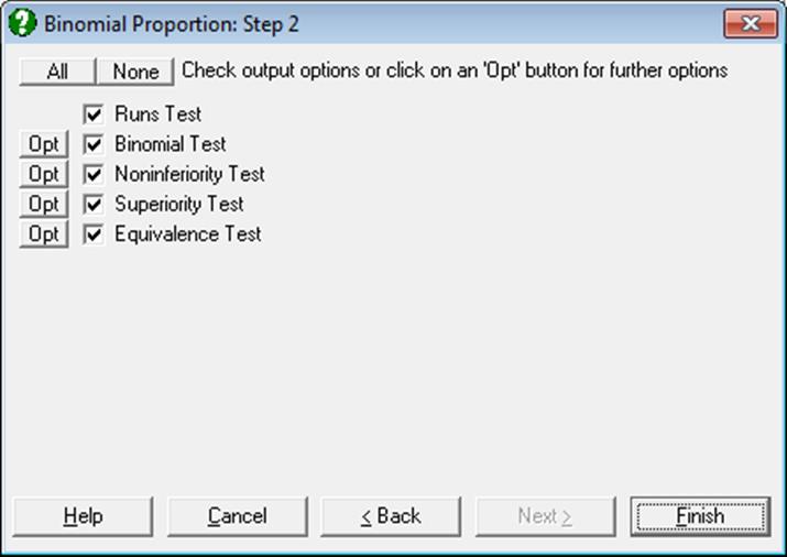
6.4.3. Binomial Proportion
One of the three data types supported for binary data can be selected (see 6.0.6. Tests with Binary Data).
You can set the value of some user-defined parameters (such as expected proportion) using the [Opt] buttons in the Output Options Dialogue. If [Finish] is clicked instead, the default value suggested by the program will be used.
6.4.3.1. Runs Test
This test is used to determine the randomness of cases belonging to two outcomes within a sample. The number of runs R (i.e. the number of groups of cases which belong to the same group) in the raw data is counted. If the last data option Test Statistics are Given is selected then an [Opt] button will also be available for Runs Test, allowing entry of a number of runs value.
Two sets of results are reported using the normal approximation.
Asymptotic without Continuity Correction: In this case the Z-statistic is defined as:
![]()
where:
![]()
![]()
Asymptotic with Continuity Correction: The Z-statistic with continuity correction is defined as:
![]()
In some applications, the test statistic with continuity
correction is reported for ![]() and without
continuity correction otherwise.
and without
continuity correction otherwise.
The output includes the number of cases in each group as well as the number of runs. The same normal approximation is also used for the Wald-Wolfowitz Runs Test.
Example
Example 25.8, p. 598 from Zar, J. H. (2010). The null hypothesis “the sequence is in a random order” is tested.
Open NONPAR12 and select Statistics 1 → Nonparametric Tests (1-2 Samples) → Binomial Proportion, the data option 1 Column Contains Two Categories. Then select Species (S15) as [Column 1] and check only the Runs Test output option to obtain the following results:
Binomial Proportion
Data option: Column Contains Two Categories
|
|
Cases |
|
Species = A |
9 |
|
Species = B |
13 |
|
Total |
22 |
Runs Test
|
|
Number of Runs |
Z-Statistic |
1-Tail Probability |
2-Tail Probability |
|
Asymptotic |
8 |
-1.4197 |
0.0779 |
0.1557 |
|
Asymptotic with CC |
|
-1.6460 |
0.0499 |
0.0998 |
This result is not significant at the 5% level (i.e. p > 0.05) and therefore do not reject the null hypothesis “the sequence is in a random order”. Note that the number of runs is given wrongly as 9 in the book.
6.4.3.2. Binomial Test
This test compares the observed ratio of two groups (e.g. successes and failures) in a sample with a given expected ratio. There are many different methods to estimate the confidence intervals and tail probabilities for a Binomial Proportion. For details see Newcombe, R. G. (1998).
It is also possible to perform this test for each binary factor in a 2 x 2 table using the Contingency Table and Cross-Tabulation procedures (see 6.6.2.3. 2 x 2 Table Statistics).
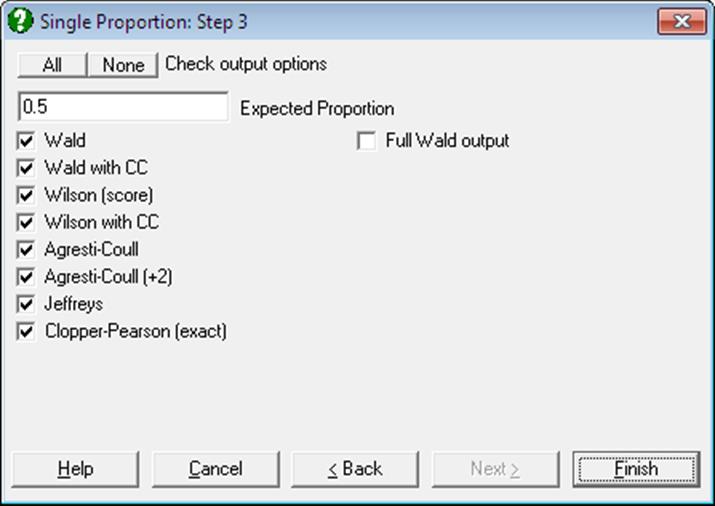
The further options dialogue is accessed by clicking on the [Opt] button situated to the left of the Binomial Test check box. By default, the program suggests an expected proportion of 0.5, however, this can be changed to any value between 0 and 1. The output includes a summary table for the number of cases in each group as well as the observed and expected ratios. You can choose to display any of the following eight more commonly used methods.
Wald: This is the standard asymptotic method without continuity correction. Confidence limits with normal approximation to binomial distribution are:
![]()
where:
![]()
is the observed proportion and:
![]()
is the sample standard error. The standard error used in confidence interval calculations is the sample standard error, which is based on the observed proportion.
On the next line, the standard error based on the null hypothesis (H0: observed proportion is equal to the expected proportion) and the corresponding one- and two-tailed normal probabilities are reported:
![]()
![]()
where p0 is the expected proportion.
If the Full Wald Output box is checked, then the missing parts of the Wald output, i.e. one- and two-tailed probabilities based on the sample standard error:
![]()
and the confidence limits under H0:
![]()
are also displayed. The user should take care with the interpretation of this extended output.
Wald with Continuity Correction: A continuity correction term of 1/(2n) is included:
![]()
In this case, the Z-statistic based on the expected proportion (the null hypothesis H0: proportion is equal to the expected proportion) is:
![]()
If the Full Wald Output box is checked, then the missing parts of the Wald output, i.e. one- and two-tailed probabilities based on the sample standard error and the confidence limits under H0 are also displayed. The user should take care with the interpretation of this extended output.
Wilson (score): The confidence limits without continuity correction are:
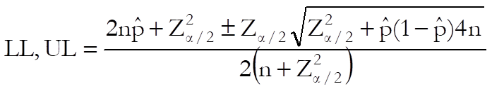
Earlier versions of UNISTAT report these confidence limits for the Asymptotic without Continuity Correction case.
Wilson with Continuity Correction:
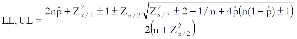
Earlier versions of UNISTAT report these confidence limits for the Asymptotic with Continuity Correction case.
Agresti-Coull: This is similar to Wald interval but ![]() (i.e.
half of the square of normal critical value) is added to numbers of successes
and failures:
(i.e.
half of the square of normal critical value) is added to numbers of successes
and failures:
![]()
where:
![]()
![]()
![]()
![]()
If the Full Wald Output box is checked, then the following Z-statistic and its one- and two-tailed probabilities are also displayed:
![]()
Agresti-Coull (+2): This
similar to the Agresti-Coull interval except that 2 (a crude approximation to ![]() ) is added to the numbers of successes
and failures:
) is added to the numbers of successes
and failures:
![]()
![]()
![]()
If the Full Wald Output box is checked, then the following Z-statistic and its one- and two-tailed probabilities are also displayed:
![]()
Jeffreys: The confidence limits are defined as the following critical values from the inverse beta distribution:
![]()
![]()
Clopper-Pearson (exact): The exact one- and two-tailed binomial probabilities are reported. The exact confidence interval is calculated as:
![]()
![]()
Example 1
Table I on p. 861 from Newcombe, R. G. (1998) where examples with five confidence intervals supported by UNISTAT are given. The following group sizes are given for the second column of the results table.
|
Size of Group 1 |
15 |
|
Size of Group 2 |
133 |
|
Expected Proportion |
0.5 |
Select Statistics 1 → Nonparametric Tests (1-2 Samples) → Binomial Proportion and select the data option 3 Cell Frequencies are Given. Enter the above group sizes and check only the Binomial Test output option to obtain the following results:
Binomial Proportion
Data option: Test Statistics are Given
|
|
Cases |
|
Group 1 |
15 |
|
Group 2 |
133 |
|
Total |
148 |
Binomial Test
|
Expected Proportion = |
0.5000 |
|
Observed Proportion = |
0.1014 |
|
|
Proportion used in SE |
Standard Error |
Z-Statistic |
1-Tail Probability |
2-Tail Probability |
|
Wald |
0.1014 |
0.0248 |
|
|
|
|
H0 |
0.5000 |
0.0411 |
-9.6995 |
0.0000 |
0.0000 |
|
Wald with CC |
0.1014 |
0.0248 |
|
|
|
|
H0 |
0.5000 |
0.0411 |
-9.6173 |
0.0000 |
0.0000 |
|
Wilson (score) |
|
|
|
|
|
|
Wilson with CC |
|
|
|
|
|
|
Agresti-Coull |
0.1114 |
0.0255 |
|
|
|
|
Agresti-Coull (+2) |
0.1118 |
0.0256 |
|
|
|
|
Jeffreys |
|
|
|
|
|
|
Clopper-Pearson (exact) |
|
|
|
0.0000 |
0.0000 |
|
|
Lower 95% |
Upper 95% |
|
Wald |
0.0527 |
0.1500 |
|
H0 |
|
|
|
Wald with CC |
0.0494 |
0.1534 |
|
H0 |
|
|
|
Wilson (score) |
0.0624 |
0.1605 |
|
Wilson with CC |
0.0598 |
0.1644 |
|
Agresti-Coull |
0.0614 |
0.1615 |
|
Agresti-Coull (+2) |
0.0617 |
0.1619 |
|
Jeffreys |
0.0604 |
0.1576 |
|
Clopper-Pearson (exact) |
0.0578 |
0.1617 |
Example 2
Example 4.6 on p. 115 from Armitage & Berry (2002). Patients’ preference for two analgesic drugs, X and Y is recorded. The null hypothesis “the ratio of preferences is not different from 50%” is tested.
|
Size of Group 1 |
65 |
|
Size of Group 2 |
35 |
|
Expected Proportion |
0.5 |
Select Statistics 1 → Nonparametric Tests (1-2 Samples) → Binomial Proportion and select the data option 3 Cell Frequencies are Given. Enter values in the above table and check only the Binomial Test output option to obtain the following results:
Binomial Proportion
Data option: Test Statistics are Given
|
|
Cases |
|
Group 1 |
65 |
|
Group 2 |
35 |
|
Total |
100 |
Binomial Test
|
Expected Proportion = |
0.5000 |
|
Observed Proportion = |
0.6500 |
|
|
Proportion used in SE |
Standard Error |
Z-Statistic |
1-Tail Probability |
2-Tail Probability |
|
Wald |
0.6500 |
0.0477 |
|
|
|
|
H0 |
0.5000 |
0.0500 |
3.0000 |
0.0013 |
0.0027 |
|
Wald with CC |
0.6500 |
0.0477 |
|
|
|
|
H0 |
0.5000 |
0.0500 |
2.9000 |
0.0019 |
0.0037 |
|
Wilson (score) |
|
|
|
|
|
|
Wilson with CC |
|
|
|
|
|
|
Agresti-Coull |
0.6445 |
0.0470 |
|
|
|
|
Agresti-Coull (+2) |
0.6442 |
0.0469 |
|
|
|
|
Jeffreys |
|
|
|
|
|
|
Clopper-Pearson (exact) |
|
|
|
0.0018 |
0.0035 |
|
|
Lower 95% |
Upper 95% |
|
Wald |
0.5565 |
0.7435 |
|
H0 |
|
|
|
Wald with CC |
0.5515 |
0.7485 |
|
H0 |
|
|
|
Wilson (score) |
0.5525 |
0.7364 |
|
Wilson with CC |
0.5474 |
0.7409 |
|
Agresti-Coull |
0.5524 |
0.7365 |
|
Agresti-Coull (+2) |
0.5522 |
0.7362 |
|
Jeffreys |
0.5533 |
0.7382 |
|
Clopper-Pearson (exact) |
0.5482 |
0.7427 |
This result is significant at the 1% level. Hence reject the null hypothesis “the patients have no significant preference for a particular analgesic drug”.
6.4.3.3. Noninferiority Test
The null hypothesis tested is that “the expected proportion is worse than the expected proportion by a given margin δ”. The alternative hypothesis is “the observed proportion is not inferior.”
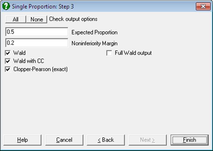
The noninferiority test similar to Binomial Test with the exception that the expected proportion is reduced by the noninferiority margin δ. Also, the Z-statistic is based on the observed proportion (unlike the Binomial Test where it is based on the expected proportion H0). The confidence limits are reported at 1 – 2α level, rather than the usual 1 – α.
Wald: By default, the Z-statistic and the confidence interval are both based on the sample standard error:
![]()
![]()
where:
![]()
is the observed proportion and:
![]()
and:
![]()
If the Full Wald Output box is checked, then on the next line, the Z-statistic and confidence interval based on the noninferiority limit are also reported:
![]()
![]()
where:
![]()
Wald with Continuity Correction: A continuity correction term of 1/(2n) is included as in the Binomial Test.
Clopper-Pearson (exact): The exact one- and two-tailed binomial probabilities and the exact confidence interval are reported.
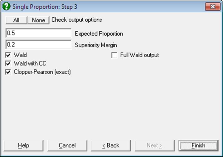
6.4.3.4. Superiority Test
This is identical to Noninferiority Test except that the given margin δ is added to the expected proportion, rather than subtracted.
6.4.3.5. Equivalence Test for Binomial Proportion
This is, in effect, a combined Noninferiority Test and Superiority Test. An overall test table displays the larger one-tail probability comparing the two tests and their corresponding lower and upper confidence limits.
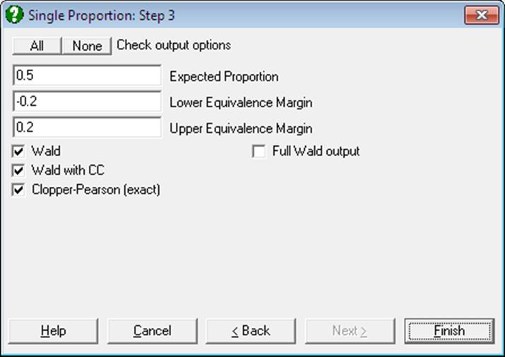
This is the nonparametric version of equivalence test for means (see 6.1.2. Equivalence Test for Means).
Example 1
|
Size of Group 1 |
228 |
|
Size of Group 2 |
534 |
Select Statistics 1 → Nonparametric Tests (1-2 Samples) → Binomial Proportion and select the data option 3 Cell Frequencies are Given. Enter the above group sizes (and enter 1 for the Number of Runs to proceed) and click on the [Opt] button for the Equivalence Test output option. Enter the following and click [Finish]:
|
Expected Proportion |
0.28 |
|
Lower Equivalence Margin |
-0.1 |
|
Upper Equivalence Margin |
0.1 |
Binomial Proportion
Data option: Test Statistics are Given
|
|
Cases |
|
Group 1 |
228 |
|
Group 2 |
534 |
|
Total |
762 |
Equivalence Test
|
Expected Proportion = |
0.2800 |
|
Observed Proportion = |
0.2992 |
|
Lower Equivalence Margin = |
-0.1000 |
|
Lower Equivalence |
Proportion used in SE |
Standard Error |
Z-Statistic |
1-Tail Probability |
2-Tail Probability |
|
Wald |
0.2992 |
0.0166 |
7.1865 |
0.0000 |
|
|
H0 |
0.1800 |
|
|
|
|
|
Wald with CC |
0.2992 |
0.0166 |
7.1469 |
0.0000 |
|
|
H0 |
0.1800 |
|
|
|
|
|
Clopper-Pearson (exact) |
|
|
|
0.0000 |
|
|
Lower Equivalence |
Lower 90% |
Upper 90% |
|
Wald |
0.2719 |
|
|
H0 |
|
|
|
Wald with CC |
0.2713 |
|
|
H0 |
|
|
|
Clopper-Pearson (exact) |
0.2719 |
|
|
Upper Equivalence Margin = |
0.1000 |
|
Upper Equivalence |
Proportion used in SE |
Standard Error |
Z-Statistic |
1-Tail Probability |
2-Tail Probability |
|
Wald |
0.2992 |
0.0166 |
-4.8701 |
0.0000 |
|
|
H0 |
0.3800 |
|
|
|
|
|
Wald with CC |
0.2992 |
0.0166 |
-4.8305 |
0.0000 |
|
|
H0 |
0.3800 |
|
|
|
|
|
Clopper-Pearson (exact) |
|
|
|
0.0000 |
|
|
Upper Equivalence |
Lower 90% |
Upper 90% |
|
Wald |
|
0.3265 |
|
H0 |
|
|
|
Wald with CC |
|
0.3272 |
|
H0 |
|
|
|
Clopper-Pearson (exact) |
|
0.3277 |
|
Overall |
1-Tail Probability |
Lower 90% |
Upper 90% |
|
Wald |
0.0000 |
0.2719 |
0.3265 |
|
Wald with CC |
0.0000 |
0.2713 |
0.3272 |
|
Clopper-Pearson (exact) |
0.0000 |
0.2719 |
0.3277 |