6.1.1. t- and F-Tests
All t- and F-Tests can be accessed under this menu item and the results presented in a single page of output.
If you wish to perform a One Sample t-Test, you can select only one variable. If you select two or more variables, then for each pair, two separate one sample t-tests will be performed on each variable, alongside the two sample tests between them. A paired t-test will be performed only when the two selected variables have the same size. Output Options Dialogue will allow you to choose which tests to appear in the output.
The t-test is used to determine whether the difference between two means is significant. The null hypothesis tested in all four types of t-test is that “the difference between two population means is zero”. When the alternative hypothesis is “the difference is not equal to zero”, the two-tailed probability should be compared against the given significance level α (usually 0.05). If the calculated probability is greater than α, then the null hypothesis cannot be rejected. Otherwise, we can conclude that the two means are significantly different. In this case, the confidence interval for the difference will not enclose 0. When the alternative hypothesis is a difference in one direction (i.e. one mean is greater or less than the other), then the one-tailed probability is compared against α. UNISTAT reports both one and two-tailed probabilities, where the former is the half of the latter.
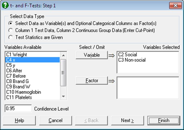
The data for this test can be in one of the three types supported for Two Sample Tests.
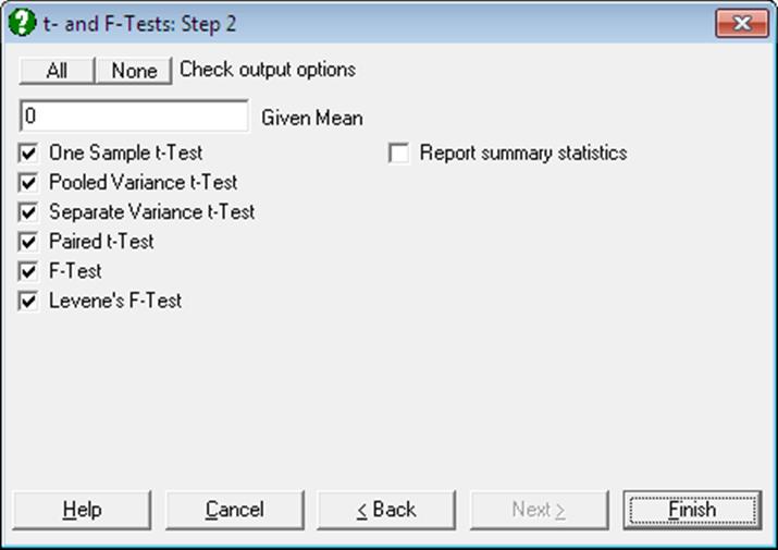
After the variable selection is complete, you will be able to select which tests you wish to have displayed in the output. The output consists of the t-value, its degrees of freedom, one and two-tailed probabilities and the confidence interval for the specified confidence level. When the Report summary statistics box is checked, summary information (number of valid cases, missing observations or pairs, mean and standard deviation) about the selected variables is also displayed.
6.1.1.1. One Sample t-Test
If only one variable is selected, the program will perform only a one-sample t-test against the given mean. By default, the given mean is 0, testing whether the mean of the sample is different from zero. If two or more variables have been selected, then the program will perform two separate one-sample t-tests on each pair of variables, using the same given mean specified in the Output Options Dialogue. Missing cases are omitted by case and the degrees of freedom is adjusted accordingly.
The null hypothesis that “the population mean is equal to the given mean” (a scalar) is tested. The population variance is assumed to be unknown. The t-statistic is computed as:
![]()
![]()
where M is the given mean.
Example
Example 4.2 on p. 101 from Armitage & Berry (2002). The null hypothesis “the population mean is not significantly different from 24” is tested at 95% and 99% levels.
Open PARTESTS, select Statistics 1 → Parametric Tests → t- and F-Tests, select the first column Weight (C1) as [Variable] and click [Next]. Type 24 into the Given Mean box, select all output options (including the Report summary statistics box) and click [Next] to obtain the following results:
t- and F-Tests
For Weight
|
|
Valid Cases |
Missing |
Mean |
Standard Deviation |
Difference |
Standard Error |
|
Mean(Weight) – 24 |
20 |
0 |
21.0000 |
5.9116 |
-3.0000 |
1.3219 |
|
|
t-Statistic |
Degrees of Freedom |
1-Tail Probability |
2-Tail Probability |
Lower 95% |
Upper 95% |
|
Mean(Weight) – 24 |
-2.2695 |
19.0000 |
0.0175 |
0.0351 |
-5.7667 |
-0.2333 |
Since the two-tailed probability is less than 5% we reject the null hypothesis and conclude that the population mean is significantly different from 24 at a 95% level. The same result can also be obtained from the reported confidence interval for the difference between means (-5.7667 to -0.2333), since it does not include zero.
If, however, the confidence level is increased to 99%, the null hypothesis should not be rejected, as the two-tailed probability is greater than 1%. This can also be observed from the confidence interval by repeating the test with a 99% confidence level. Select the test again and edit the Confidence Level box to 0.99 in Variable Selection Dialogue. This time, the confidence interval includes zero.
|
|
Lower 99% |
Upper 99% |
|
Mean(Weight) – 24 |
-6.7818 |
0.7818 |
6.1.1.2. Pooled Variance t-Test
The null hypothesis “two population means are equal” is tested. It is assumed that the two populations are independent and their standard deviations are the same. The assumption of equal variances can be tested by using the F-test or Levene’s F-Test, which is part of the standard output of this procedure. If the two-tailed probability for the F-value is greater than the specified α (such as 0.01 or 0.05), then the hypothesis of equal variances is not rejected and the t-test can use the pooled-variance estimate (equal variances). Otherwise the t-test should be based on separate variance estimates (unequal variances).
The t-statistic for equal population variances is calculated as follows:
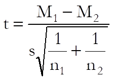
![]()
where:
![]()
is the pooled estimate of the population variance.
Missing values are omitted by case and the degrees of freedom is adjusted accordingly.
Example 1
Table 87 on p. 231 from Cohen, L. & M. Holliday (1983). The null hypothesis “empathy scores of social and non-social work students have the same mean” is tested at a 95% confidence level.
Open PARTESTS and select Statistics 1 → Parametric Tests → t- and F-Tests. Select the data option 1 and Social and Non-social (C2 and C3) as [Variable]s. Enter 0 for the Given Mean and select all output options. The following results are obtained:
t- and F-Tests
For Social and Non-social
|
|
Valid Cases |
Missing |
Mean |
Standard Deviation |
|
Mean(Social) – 0 |
10 |
0 |
75.5000 |
4.5031 |
|
Mean(Non-social) – 0 |
10 |
0 |
63.1000 |
5.9712 |
|
Pooled Variance |
|
|
|
5.2884 |
|
Separate Variance |
|
|
|
|
|
Paired |
10 |
0 |
|
5.2957 |
|
|
Difference |
Standard Error |
t-Statistic |
Degrees of Freedom |
|
Mean(Social) – 0 |
75.5000 |
1.4240 |
53.0196 |
9.0000 |
|
Mean(Non-social) – 0 |
63.1000 |
1.8883 |
33.4169 |
9.0000 |
|
Pooled Variance |
12.4000 |
2.3650 |
5.2431 |
18.0000 |
|
Separate Variance |
12.4000 |
2.3650 |
5.2431 |
16.7351 |
|
Paired |
12.4000 |
1.6746 |
7.4045 |
9.0000 |
|
|
1-Tail Probability |
2-Tail Probability |
Lower 95% |
Upper 95% |
|
Mean(Social) – 0 |
0.0000 |
0.0000 |
72.2787 |
78.7213 |
|
Mean(Non-social) – 0 |
0.0000 |
0.0000 |
58.8284 |
67.3716 |
|
Pooled Variance |
0.0000 |
0.0001 |
7.4313 |
17.3687 |
|
Separate Variance |
0.0000 |
0.0001 |
7.4042 |
17.3958 |
|
Paired |
0.0000 |
0.0000 |
8.6117 |
16.1883 |
|
|
Variance 1 |
Variance 2 |
F-Statistic |
d.f. Numerator |
d.f. Denominator |
|
F-Test |
20.2778 |
35.6556 |
1.7584 |
9 |
9 |
|
Levene’s F Test |
|
|
0.6515 |
1 |
18 |
|
|
Right-Tail Probability |
2-Tail Probability |
Lower 95% |
Upper 95% |
|
F-Test |
0.2066 |
0.4132 |
0.4368 |
7.0791 |
|
Levene’s F Test |
|
0.4301 |
|
|
This result shows that there is a significant difference at the 0.1% level, between the empathy scores of social work students and non-social work students.
Example 2
Example on p. 30, Gardner & Altman (2000). Blood pressure level data for diabetics and non diabetics are not available but all necessary parameters to perform a t-test are given.
|
Size of Group 1 |
100 |
|
Size of Group 2 |
100 |
|
Mean 1 |
146.4 |
|
Mean 2 |
140.4 |
|
Standard Deviation 1 |
18.5 |
|
Standard Deviation 2 |
16.8 |
Select Statistics 1 → Parametric Tests → t- and F-Tests, select the data option 3 Test Statistics are Given and enter the above data. Leave the default value of the confidence level unchanged at 0.95. Check all output options except the Report summary statistics box. The following results are obtained:
t- and F-Tests
Test Statistics are Given
|
|
Difference |
Standard Error |
t-Statistic |
Degrees of Freedom |
|
Mean(Group 1) – 0 |
146.4000 |
1.8500 |
79.1351 |
99.0000 |
|
Mean(Group 2) – 0 |
140.4000 |
1.6800 |
83.5714 |
99.0000 |
|
Pooled Variance |
6.0000 |
2.4990 |
2.4010 |
198.0000 |
|
Separate Variance |
6.0000 |
2.4990 |
2.4010 |
196.1884 |
|
|
1-Tail Probability |
2-Tail Probability |
Lower 95% |
Upper 95% |
|
Mean(Group 1) – 0 |
0.0000 |
0.0000 |
142.7292 |
150.0708 |
|
Mean(Group 2) – 0 |
0.0000 |
0.0000 |
137.0665 |
143.7335 |
|
Pooled Variance |
0.0086 |
0.0173 |
1.0720 |
10.9280 |
|
Separate Variance |
0.0086 |
0.0173 |
1.0717 |
10.9283 |
|
|
F-Statistic |
d.f. Numerator |
d.f. Denominator |
|
F-Test |
1.2126 |
99 |
99 |
|
|
Right-Tail Probability |
2-Tail Probability |
Lower 95% |
Upper 95% |
|
F-Test |
0.1696 |
0.3391 |
0.8159 |
1.8022 |
Note that paired t-test and Levene’s F-Test cannot be computed when the data option Test Statistics are Given is selected.
Next, click on the [Last Procedure Dialogue] button to re-display the Variable Selection Dialogue. Edit the value of the confidence level to 0.99 and click [Finish]. All results will be as above except for the confidence intervals. The interval for pooled variance t-test will be:
|
|
Lower 99% |
Upper 99% |
|
Pooled Variance |
-0.4996 |
12.4996 |
And finally, edit the confidence level to 0.9 and repeat the procedure to obtain:
|
|
Lower 90% |
Upper 90% |
|
Pooled Variance |
1.8702 |
10.1298 |
6.1.1.3. Separate Variance t-Test
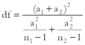
The null hypothesis “the means of two populations are equal” is tested. It is assumed that their standard deviations may be different. The resulting t-statistic is based on a number of degrees of freedom which is reduced by a factor depending on the extent of the differences in variances.
![]()
where:
and where:
![]()
The reported degrees of freedom (Satterthwaite’s approximation) may not be an integer but the nearest integer is used to calculate the tail probabilities.
Missing values are omitted by case and the degrees of freedom is adjusted accordingly.
Example
Table 89 on p. 233 from Cohen, L. & M. Holliday (1983). The raw data on social perceptiveness scores of nursery school and non-nursery school children are not available, but all parameters necessary to perform a t-test are given.
|
Size of Group 1 |
71 |
|
Size of Group 2 |
64 |
|
Mean 1 |
19.5 |
|
Mean 2 |
15.3 |
|
Standard Deviation 1 |
3.4 |
|
Standard Deviation 2 |
4.6 |
Select Statistics 1 → Parametric Tests → t- and F-Tests. Select the data option 3 Test Statistics are Given and enter the above values. Check only the Separate Variance t-test output option to obtain the following results:
t- and F-Tests
Test Statistics are Given
|
|
Difference |
Standard Error |
t-Statistic |
Degrees of Freedom |
|
Separate Variance |
4.2000 |
0.7025 |
5.9790 |
115.1866 |
|
|
1-Tail Probability |
2-Tail Probability |
Lower 95% |
Upper 95% |
|
Separate Variance |
0.0000 |
0.0000 |
2.8086 |
5.5914 |
This result shows that there is a significant difference at the 0.1% level, of the social perceptiveness of nursery school and non-nursery school children.
6.1.1.4. Paired t-Test
This test will be available only when the following conditions are met:
· The data option 1 is selected
· At least two variables are selected
· The selected pairs have the same length.
Two or more columns can be selected by clicking on [Variable]. The test will be performed between all possible pairs, as long as the two columns have the same size. For each test, any pair of cases with one or more missing values is omitted and the degrees of freedom adjusted. It is also possible to perform t-tests between subgroups of two variables defined by one or more factor columns. In this case, the Run a separate analysis for each option selected box must be unchecked.
A paired t-test is performed between two variables, such as values of a sample before and after a certain treatment. The null hypothesis tested is “the difference between pairs is zero” against the alternative hypothesis that “the difference between pairs is not equal to zero”.
The t-statistic is calculated as follows:
![]()
![]()
where MD and sD are the mean and standard error of D and:
![]()
Example 1
Example 8.3.4 on pp. 454-54, Larson, H. J. (1982). The null hypothesis “reaction times before consumption of beverage x and after consumption y on individuals are equal” is tested.
Open PARTESTS and select Statistics 1 → Parametric Tests → t- and F-Tests. Select x and y (C4 and C5) as [Variable]s and check only the One-sample t-test and Paired t-test boxes to obtain the following results:
t- and F-Tests
For x and y
|
|
Difference |
Standard Error |
t-Statistic |
Degrees of Freedom |
|
Mean(x) – 0 |
602.4000 |
29.3342 |
20.5358 |
9.0000 |
|
Mean(y) – 0 |
803.7000 |
19.6413 |
40.9190 |
9.0000 |
|
Paired |
-201.3000 |
15.1056 |
-13.3262 |
9.0000 |
|
|
1-Tail Probability |
2-Tail Probability |
Lower 95% |
Upper 95% |
|
Mean(x) – 0 |
0.0000 |
0.0000 |
536.0415 |
668.7585 |
|
Mean(y) – 0 |
0.0000 |
0.0000 |
759.2684 |
848.1316 |
|
Paired |
0.0000 |
0.0000 |
-235.4712 |
-167.1288 |
This result shows that there is a significant difference at the 5% level, of the reaction time of individuals before and after consumption of beverage.
Example 2
Example on p. 31, Gardner & Altman (2000). Data on testing the difference between the systolic blood pressure levels for 16 middle aged men before and after a standard exercise are given. The difference between the two columns should be in the order of After – Before.
Open PARTESTS and select Statistics 1 → Parametric Tests → t- and F-Tests and select Before and After (C6 and C7) as [Variable]s and check all output options to obtain the following results:
t- and F-Tests
For After and Before
|
|
Valid Cases |
Missing |
Mean |
Standard Deviation |
|
Mean(After) – 0 |
16 |
0 |
147.7500 |
12.3477 |
|
Mean(Before) – 0 |
16 |
0 |
141.1250 |
13.6229 |
|
Pooled Variance |
|
|
|
13.0010 |
|
Separate Variance |
|
|
|
|
|
Paired |
16 |
0 |
|
5.9652 |
|
|
Difference |
Standard Error |
t-Statistic |
Degrees of Freedom |
|
Mean(After) – 0 |
147.7500 |
3.0869 |
47.8630 |
15.0000 |
|
Mean(Before) – 0 |
141.1250 |
3.4057 |
41.4376 |
15.0000 |
|
Pooled Variance |
6.6250 |
4.5965 |
1.4413 |
30.0000 |
|
Separate Variance |
6.6250 |
4.5965 |
1.4413 |
29.7148 |
|
Paired |
6.6250 |
1.4913 |
4.4425 |
15.0000 |
|
|
1-Tail Probability |
2-Tail Probability |
Lower 95% |
Upper 95% |
|
Mean(After) – 0 |
0.0000 |
0.0000 |
141.1704 |
154.3296 |
|
Mean(Before) – 0 |
0.0000 |
0.0000 |
133.8659 |
148.3841 |
|
Pooled Variance |
0.0799 |
0.1599 |
-2.7624 |
16.0124 |
|
Separate Variance |
0.0800 |
0.1600 |
-2.7662 |
16.0162 |
|
Paired |
0.0002 |
0.0005 |
3.4464 |
9.8036 |
|
|
Variance 1 |
Variance 2 |
F-Statistic |
d.f. Numerator |
d.f. Denominator |
|
F-Test |
152.4667 |
185.5833 |
1.2172 |
15 |
15 |
|
Levene’s F Test |
|
|
0.1228 |
1 |
30 |
|
|
Right-Tail Probability |
2-Tail Probability |
Lower 95% |
Upper 95% |
|
F-Test |
0.3542 |
0.7084 |
0.4253 |
3.4838 |
|
Levene’s F Test |
|
0.7284 |
|
|
6.1.1.5. F-Test
The F-Test is used to compare
variances or standard deviations of two samples. The null hypothesis tested is
“the two populations have equal variances”. Columns selected for this test need
not be equal in size. Output displays the F-value, degrees of freedom, the right
and two-tailed probabilities from the F-distribution and the confidence
interval for the specified confidence level. When the alternative hypothesis is
“the two population variances are not equal”, use the two-tailed probability. When
![]() the F-value is calculated as follows:
the F-value is calculated as follows:
![]()
![]()
![]()
If ![]() then the F-value is
inverted and the two degrees of freedom are interchanged. In other words, the F-value
is always the larger variance divided by the smaller variance.
then the F-value is
inverted and the two degrees of freedom are interchanged. In other words, the F-value
is always the larger variance divided by the smaller variance.
Example 1
Example 5.1 on p. 151 from Armitage & Berry (2002). The null hypothesis “the two population variances are not significantly different” is tested at 95% level. The raw data are not available, but it is sufficient to know the number of cases in each group and their variances to perform an F-test .
|
Size of Group 1 |
10 |
|
Size of Group 2 |
20 |
|
Variance 1 |
1.232 |
|
Variance 2 |
0.304 |
Select Statistics 1 → Parametric Tests → t- and F-Tests, the data option 3 Test Statistics are Given. As this dialogue asks for standard deviations rather than variances, enter Sqr(1.232) and Sqr(0.304) for the two standard deviations. The mean values are not used for F-test. In the Output Options Dialogue, check only the F-test and Levene’s F-Test boxes. The following results are obtained:
t- and F-Tests
Test Statistics are Given
|
|
F-Statistic |
d.f. Numerator |
d.f. Denominator |
|
F-Test |
4.0526 |
9 |
19 |
|
|
Right-Tail Probability |
2-Tail Probability |
Lower 95% |
Upper 95% |
|
F-Test |
0.0049 |
0.0099 |
1.4071 |
14.9272 |
Since the null hypothesis suggests a two-tailed test (equal vs. not equal) then the two-tailed probability should be compared with α. This result shows there is no significant difference between the two population variances at 5% level for the two-tailed test.
When the data option 3 Test Statistics are Given is selected the Levene’s test cannot be computed.
Example 2
Example 8.3.2 on pp. 450-51, Larson, H. J. (1982). The null hypothesis “the population variances for hours of services given by 60 watt light bulbs of brand G and brand W are the same” is tested.
Open PARTESTS and select Statistics 1 → Parametric Tests → t- and F-Tests. Select Brand G and Brand W (C8 and C9) as [Variable]s and check only the F-test, Levene’s F-Test and Report summary statistics boxes to obtain the following results:
t- and F-Tests
For Brand G and Brand W
|
|
Variance 1 |
Variance 2 |
F-Statistic |
d.f. Numerator |
d.f. Denominator |
|
F-Test |
2222.2143 |
653.8778 |
3.3985 |
7 |
9 |
|
Levene’s F Test |
|
|
1.4112 |
1 |
16 |
|
|
Right-Tail Probability |
2-Tail Probability |
Lower 95% |
Upper 95% |
|
F-Test |
0.0459 |
0.0917 |
0.8097 |
16.3918 |
|
Levene’s F Test |
|
0.2522 |
|
|
Since the null hypothesis suggests a two-tailed test (equal vs. not equal) then we should look at the 2-tail probability. This result shows that there is no significant difference between the two population variances at 5% level.
6.1.1.6. Levene’s F-Test
Levene’s F-Test has the advantage of being less sensitive to deviations from normality and is considered to be more powerful than the classical F-test. The alternative hypothesis for Levene’s test is “the two population variances are not equal” and the probability reported is comparable to the two-tailed probability for the F-test. The test statistic, which has an F-distribution, is computed as follows:
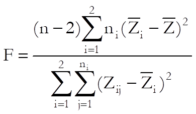
![]()
![]()
where:
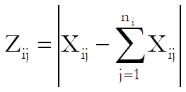
![]()
![]()
Missing values are omitted by case. If the data option 3 Test Statistics are Given is selected then the Levene’s test will not be available.