8.7. Reliability Analysis
Reliability Analysis is used to create a measurement scale for a number of variables none of which is representative of the complete group on their own. A number of reliability coefficients are computed to construct the sum scales.
Reliability Analysis is an attempt to find the true score using a set of items. These items are believed to reflect the true score and would involve some random error. The sum of these items (called the sum scale) will give an indication of the true score. The mean value of the error terms across the items will be zero. The true score component remains the same when summing across items. Therefore, the more items that are added, the more true score (relative to the error score) will be reflected in the sum scale.
The assessment of scale reliability is based on the correlation between the individual items or measurements that make up the scale, relative to the variances of the items.
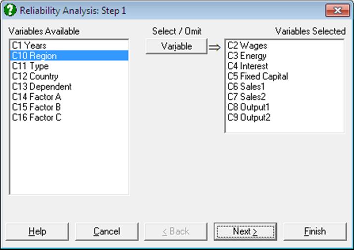
The columns containing the items are selected by clicking on [Variable]. Any rows containing one or more missing values are removed from the analysis.
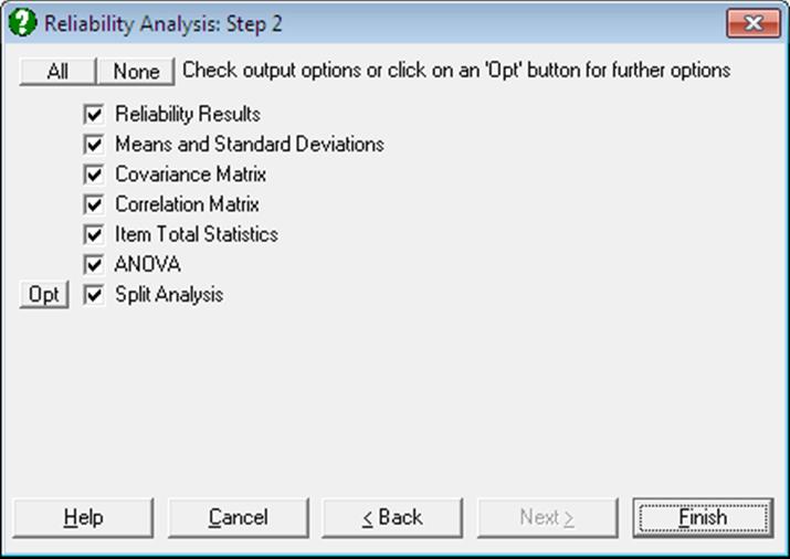
Reliability Results: The output will display summary information about the sum scale and the items. It will also display the Cronbach’s alpha statistic.
The variance of the sum scale will be smaller than the sum of item variances if the items measure the same variability. We can estimate the proportion of true score variance in the sum scale by comparing the sum of item variance with the variance of the sum scale. If the items have no error and measure the true score then alpha will equal 1. If the items are unrelated then alpha will equal 0. Standardised alpha is the value of alpha if the items had been standardised before the Reliability Analysis.
Means and Standard Deviations: The mean and standard deviation of each item is displayed.
Covariance Matrix: The covariance between the items is displayed.
Correlation Matrix: The correlation between the items is displayed.
Item Total Statistics: Sum statistics relating to each item are displayed. The first two columns contain the mean and variance that the sum scale would take if the item was removed from the scale. The third column shows the correlation between the item and the sum scale with the item removed. The final column shows the value of Cronbach’s alpha if the item was removed from the scale.
ANOVA: A one way repeated measures ANOVA table is displayed where the items (columns) are the levels of the factor and the rows are the repeated measures (subjects).
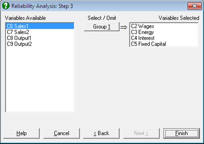
Split Analysis: The items are split into two groups. Select the items for group one by clicking on [Group 1]. The remaining items are placed in group two. If the sum scale is reliable, the two groups should be highly correlated. Split analysis calculates sum scale statistics for both groups and the correlation between the two groups.
Example
Open DEMODATA, select Statistics 2 → Reliability Analysis and select Wages to Fixed Capital (C2 to C5), Output 1 and Output 2 (C8 and C9) as [Variable]s. Select all the output options to obtain the following results.
Reliability Analysis
Variables Selected
Wages, Energy, Interest, Fixed Capital, Output1, Output2
Reliability Results
|
Statistics for |
Mean |
Variance |
Standard Deviation |
Variables |
|
Scale |
582.5786 |
3733.7172 |
61.1042 |
6 |
|
Statistics for |
Mean |
Minimum |
Maximum |
Variance |
|
Item Mean |
97.0964 |
84.1014 |
107.3121 |
105.2151 |
|
Item Variance |
128.4060 |
44.8069 |
214.6677 |
4778.0683 |
|
Covariance |
98.7760 |
23.3530 |
186.6305 |
2706.6123 |
|
Correlation |
0.7996 |
0.5141 |
0.9653 |
0.0176 |
|
Number of Cases = |
56 |
|
Cronbach’s Alpha = |
0.9524 |
|
Standardised Alpha = |
0.9599 |
Means and Standard Deviations
|
Item |
Mean |
Standard Deviation |
|
Wages |
101.9893 |
13.1962 |
|
Energy |
100.9995 |
14.6515 |
|
Interest |
84.1995 |
12.1420 |
|
Fixed Capital |
84.1014 |
11.9729 |
|
Output1 |
103.9768 |
6.6938 |
|
Output2 |
107.3121 |
6.7855 |
Covariance Matrix
|
|
Wages |
Energy |
Interest |
Fixed Capital |
Output1 |
Output2 |
|
Wages |
174.1406 |
186.6305 |
149.4251 |
145.7093 |
60.4203 |
67.2986 |
|
Energy |
186.6305 |
214.6677 |
162.2643 |
165.7807 |
76.1006 |
65.4243 |
|
Interest |
149.4251 |
162.2643 |
147.4287 |
135.4810 |
61.1438 |
59.3716 |
|
Fixed Capital |
145.7093 |
165.7807 |
135.4810 |
143.3492 |
65.5625 |
57.6750 |
|
Output1 |
60.4203 |
76.1006 |
61.1438 |
65.5625 |
44.8069 |
23.3530 |
|
Output2 |
67.2986 |
65.4243 |
59.3716 |
57.6750 |
23.3530 |
46.0431 |
Correlation Matrix
|
|
Wages |
Energy |
Interest |
Fixed Capital |
Output1 |
Output2 |
|
Wages |
1.0000 |
0.9653 |
0.9326 |
0.9222 |
0.6840 |
0.7516 |
|
Energy |
0.9653 |
1.0000 |
0.9121 |
0.9450 |
0.7759 |
0.6581 |
|
Interest |
0.9326 |
0.9121 |
1.0000 |
0.9319 |
0.7523 |
0.7206 |
|
Fixed Capital |
0.9222 |
0.9450 |
0.9319 |
1.0000 |
0.8181 |
0.7099 |
|
Output1 |
0.6840 |
0.7759 |
0.7523 |
0.8181 |
1.0000 |
0.5141 |
|
Output2 |
0.7516 |
0.6581 |
0.7206 |
0.7099 |
0.5141 |
1.0000 |
Item Total Statistics
|
|
MeanDel |
VarDel |
CorrDel |
AlphaDel |
|
Wages |
480.5893 |
2340.6090 |
0.9547 |
0.9315 |
|
Energy |
481.5791 |
2206.6489 |
0.9534 |
0.9352 |
|
Interest |
498.3791 |
2450.9170 |
0.9444 |
0.9323 |
|
Fixed Capital |
498.4771 |
2449.9511 |
0.9622 |
0.9301 |
|
Output1 |
478.6018 |
3115.7501 |
0.7670 |
0.9589 |
|
Output2 |
475.2664 |
3141.4291 |
0.7181 |
0.9618 |
Scale mean, scale variance and Cronbach’s alpha denote the
values if the item is deleted from the scale.
Correlation denotes the corrected item-total correlation
ANOVA
|
Due To |
Sum of Squares |
DoF |
Mean Square |
F-stat |
Prob |
|
Between Subjects |
34225.741 |
55 |
622.286 |
|
|
|
Within Subjects |
37608.484 |
280 |
134.316 |
|
|
|
Between Measures |
29460.233 |
5 |
5892.047 |
198.854 |
0.0000 |
|
Error |
8148.251 |
275 |
29.630 |
|
|
|
Total |
71834.225 |
335 |
214.431 |
|
|
Split Analysis
Group 1
Wages, Energy, Interest
Group 2
Fixed Capital, Output1, Output2
|
|
Number of Items |
Mean |
Sum |
Standard Deviation |
Variance |
Cronbach’s Alpha |
|
Group 1 |
3 |
287.1882 |
16082.5400 |
39.1520 |
1532.8768 |
0.9753 |
|
Group 2 |
3 |
295.3904 |
16541.8600 |
22.9648 |
527.3802 |
0.8339 |
|
Correlation Between Part 1 and Part 2 = |
0.9306 |
|
Spearman Brown Split Half Reliability = |
0.9641 |
|
Guttman Split Half Reliability = |
0.8964 |