9.3.6. Process Capability Analysis
Process Capability Analysis is used to study the variation within a process. The aim is to determine how well a process meets its specification limits, by comparing the distribution of output to the desired specification limits. A process is said to be capable when a desired (high) number of output values fall within the specification limits.
The standard Process Capability Analysis is based on two important assumptions; (i) process data is normally distributed and (ii) process is in control. When the data is not normally distributed, capability analysis can still produce useful results by using nonparametric indices, or by transforming the data so that it conforms better to normal distribution than its original form. In order to find whether a process is in control, quality control charts like R and X Bar charts can be used (see 9.3.1.1. R Chart and 9.3.1.4. X Bar Chart).
9.3.6.1. Process Capability Analysis Input Options
The Variable Selection Dialogue is of the multisample type (see 6.0.4. Multisample Tests), allowing selection of multiple data and factor columns. If only one data variable and no factors are selected, then only an overall analysis is performed. Otherwise, all selected subgroups of data are pooled to form one continuous variable and an overall and a pooled sample analyses are performed.
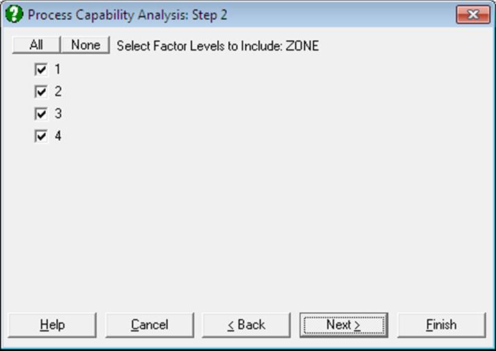
If a factor column is selected, then a further dialogue will pop up allowing you to include only the desired subgroups in the analysis. If more than one factor is selected, then all combinations of all factor levels will be listed.
9.3.6.2. Process Capability Analysis Intermediary Input Options
The next dialogue allows you to enter or edit various input parameters.
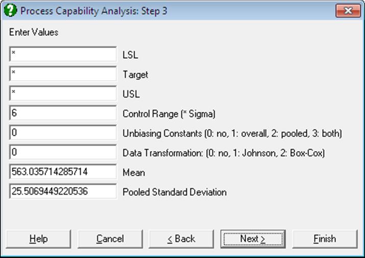
LSL: Lower Specification Limit: The smallest value below which a process is deemed not to perform satisfactorily. This value and its counterpart USL, Upper Specification Limit, are supplied by the user. If a one-sided lower specification analysis is to be carried out, then enter a single asterisk in the USL field. In this case the output will not include some indices. The program will not proceed until an LSL or USL or both are entered.
Target: Enter a value if you wish to measure the process capability performance against a target. If a value is entered, the Cpm and related indices are computed. If there is no target, enter a single asterisk in this field.
USL: Upper Specification Limit: The largest value above which a process is deemed not to perform satisfactorily. This value and its counterpart LSL, Lower Specification Limit, are supplied by the user. If a one-sided upper specification analysis is to be carried out, then enter a single asterisk in the LSL field. In this case the output will not include some indices. The program will not proceed until an LSL or USL or both are entered.
Control Range: The observed process variation in terms of sample standard deviation. This is usually 6, ± 3 sigma around the centre. If the sample is from a normally distributed population, then approximately 99% of all data points would fall within this range.
Unbiasing Constants: You can choose to apply unbiasing constants in calculations. It is possible to apply them to either or both overall and pooled standard deviations, as defined in Wheeler D. J. and Chambers D. S. (1992). The magnitude of correction gets larger as the sample size decreases.
Data Transformation: The options are 0: no transformation, 1: Johnson Transformation and 2: Box-Cox Transformation. Box-Cox Transformation will only work with positive data, whereas Johnson Transformation has no such restrictions. In most cases Johnson Transformation is more powerful than Box-Cox Transformation and it will generate transformed variables conforming better to the normal distribution. These two transformations are also available under the Statistics 2 → Quality Control → Data Transformation procedure.
The number of boxes displayed after this depends on the selection made in the Data Transformation box.
When the no transformation option is selected, one or more boxes will be displayed.
Mean: This field is available only when the no transformation option is selected. Here you can override the default mean computed from the sample and enter your own (i.e. the historical mean).
Pooled Standard Deviation: This field is available only when the no transformation option is selected and the data consists of multiple samples (i.e. if more than one variable or factor column(s) are selected). By default, the pooled sample standard deviation calculated from data is displayed. However, you can override this value and enter your own (i.e. the historical) standard deviation. If your data does not have subgroups, you can create a constant factor column (e.g. consisting of 1s) and still be able to enter a historical standard deviation.
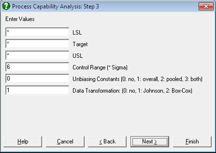
When the Johnson Transformation option is selected, there will be no further input fields.
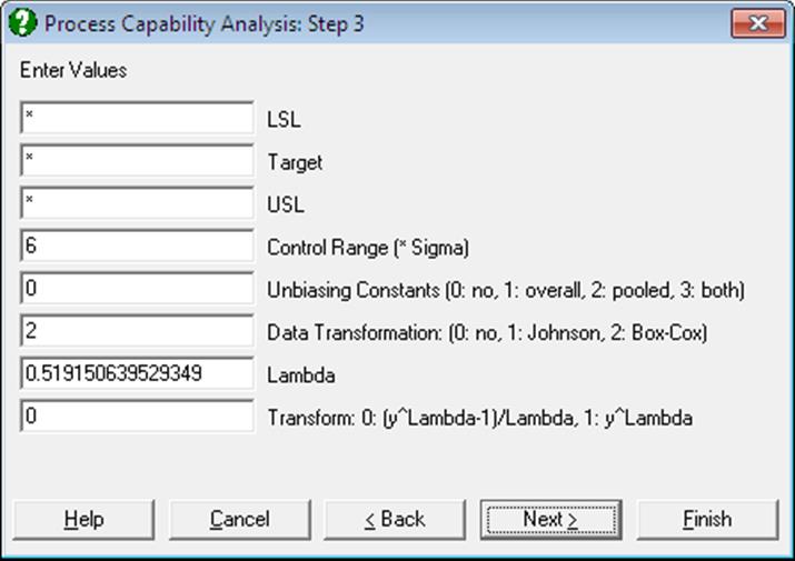
When the Box-Cox Transformation option is selected, two further input fields will be displayed, similar to ones displayed in Box-Cox Transformation (see 9.3.7.2.1 Box-Cox Transformation Intermediary Inputs).
Lambda: You can override the estimated lambda and enter your own value here. You may wish to do this to use a round power value (like -1, -0.5, 0.5, 2). If the estimated lambda is changed, confidence intervals and chi-squared tests for lambda will not be available.
Transform: Once the optimal lambda is estimated using the standard Box-Cox Transformation, you will have a chance to generate the transformed variable using, (i) the same transformation:
![]() if
if ![]()
![]() if
if ![]()
or, (ii) the simple power transformation:
![]()
In some cases the second formula may be preferable to the first, since it will not generate nonpositive values. The choice made here will not affect normality of the transformed variable.
Remember that during the maximum likelihood estimation of lambda the original variable is always transformed using the first set of equations.
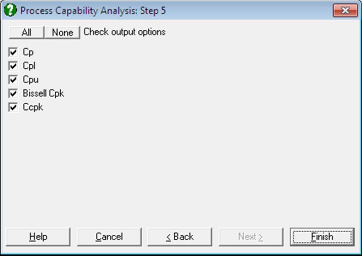
9.3.6.3. Process Capability Analysis Output Options
Some of the options displayed on this dialogue may appear disabled, depending on the choices made in previous dialogues.
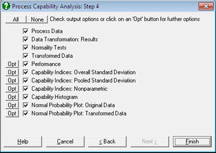
Process Data: Variables selected, summary statistics (size, mean, overall and pooled standard deviations) and parameters supplied by the user (control range, LSL target, USL) are displayed. If a Data Transformation option was selected, summary statistics for the transformed data will also be displayed.
Data Transformation Results: This option is enabled if a transformation has been selected in the previous dialogue. Optimal parameter values estimated by the program and the equation applied in transforming the dependent variable is displayed. The same equation is also printed on a separate line with estimated parameter values, in a format suitable for cell calculations in Excel. You can simply copy this equation, replace the variable x with a cell reference and run interpolations.
Normality Tests: This option is enabled if a transformation has been selected in the previous dialogue. The Anderson-Darling Test of normality is performed on the original and the transformed dependent variable thus allowing the user to judge whether the transformation was useful. No or a small increase in the tail probability indicates that the Box-Cox Transformation was not useful.
Transformed Data: This option is enabled if a transformation has been selected in the previous dialogue. The original and transformed dependent variable values and their group membership (if any) are sorted and displayed in a table.
If you are using UNISTAT in Stand-Alone Mode, click on the UNISTAT icon on the Output Medium Toolbar to send all output to UNISTAT spreadsheet. In Excel Add-In Mode select the output matrix as data for further calculations.
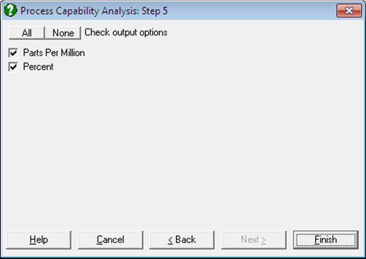
Performance: The number of cases that are expected to fall outside the specification limits is calculated and this is displayed as Parts Per Million or Percentage points.
The expected value is calculated from the cumulative normal distribution using the sample standard deviation and, in case of subgroup analysis, using both overall and pooled standard deviations.
Capability Indices: Overall Standard Deviation: Capability indices are indifferent to data transformations, since they are unitless ratios. However, when interpretation of results involves parameters in actual data units (such as standard deviation or confidence intervals), they should be transformed back into the original scale.
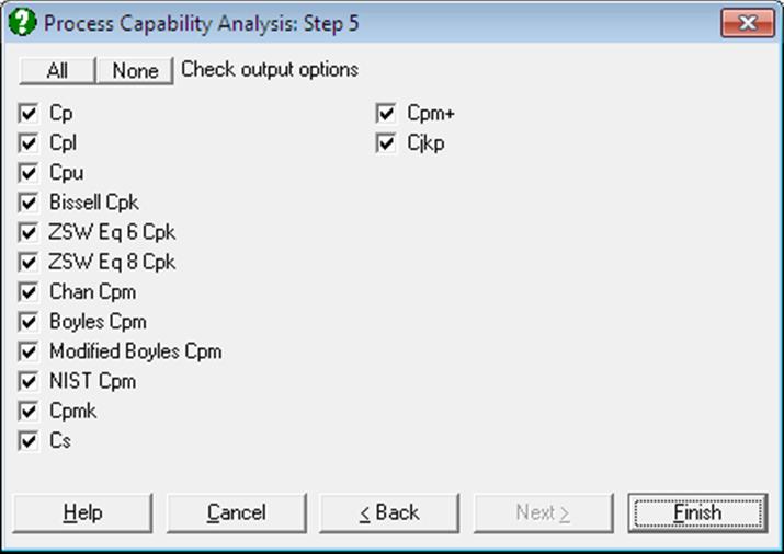
For most practical applications, many of the indices available here will be irrelevant. When this is the case, simply uncheck the unwanted options and UNISTAT will remember your choices when you run this procedure next time. You can also remove the authors’ names from the output by entering the following line in Documents\Unistat10\Unistat10.ini file under the [QC] section:
WithNames=0
Cp: Capability indices are used to compare the variability in the output of a process which is in control, to the desired specification limits. Cp is defined as the ratio of the difference between the specification limits to the control range (i.e. process variation):
![]()
It can be seen that when Cp is greater than one, the process specification covers almost all observations, as 6 sigma (the default control range) would cover approximately 99% of all data points from a normally distributed population.
The following interpretation of Cp values is widely accepted:
Cp < 1: not adequate
1 ≤ Cp ≤ 1.33: adequate
Cp > 1.33: satisfactory for existing processes
Cp > 1.50: for critical variables
Cp > 1.67: for new processes with a critical variable.
Confidence intervals for Cp are calculated as:
![]()
![]()
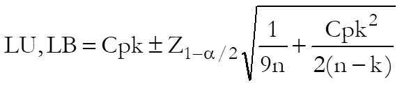
where n is the number of observations and k is the number of subgroups.
The Cp index is only available when both LSL and USL are supplied.
Cpl: This gives the capability of the lower half of the process. When USL is not available, it is still possible to determine the one-sided capability of the process:
![]()
The following interpretation of Cpl values is widely accepted:
Cpl > 1.25: satisfactory for existing processes
Cpl > 1.45: for critical variables or new processes
Cpl > 1.60: for new processes with a critical variable
The 95% confidence intervals for Cpl are calculated using the noncentral t-distribution as:
![]()
where the noncentrality parameter is:
![]()
![]()
where the noncentrality parameter is:
![]()
WARNING: Due to the iterational nature of this confidence interval algorithm, the results are accurate to about three significant digits.
Cpu: This gives the capability of the upper half of the process. When LSL is not available, it is still possible to determine the one-sided capability of the process:
![]()
The confidence intervals for Cpu are calculated in the same way as for Cpl.
Cpk: The Cp index may be misleading when the centres of the specification range and process mean are significantly different. In such cases the Cpk index, which is defined as the minimum of Cpl and Cpu, will provide a better measure:
![]()
This is the minimum distance between specification limits and the process mean divided by half of the control range.
The confidence intervals for Cpk are calculated using three different methods:
(i) Normal approximation suggested by Bissell, A. F. (1990):
(ii) Equation 6 from Zhang, N. F., Stenback, G. A., Wardrop, D. M. (1990):
![]()
where:
![]()
(iii) Equation 8 from Zhang, N. F., Stenback, G. A., Wardrop, D. M. (1990):
![]()
![]()
where:
Cpm: This index is available only when a target value is specified. It is used to measure the variability of process data around a target value. Two different methods of calculating Cpm and its confidence intervals are provided.
(i) Chan L.J., Cheng S.K., and Spiring, F.A. (1989) suggest replacing the standard deviation around the mean with deviation around the target.
![]()
When both LSL and USL are given and target level is
equal to the sample mean (i.e. ![]() ),
then:
),
then:
![]()
When both LSL and USL are given and target level is not
equal to the sample mean (i.e. ![]() ),
then:
),
then:
![]()
When LSL is given but USL is not available:
![]()
and when USL is given but LSL is not available:
![]()
The confidence intervals are given as:
![]()
![]()
where the degrees of freedom is:
and:
![]()
When both LSL and USL are given and target level is
equal to the sample mean (i.e. ![]() ),
then the one-sided alpha is used:
),
then the one-sided alpha is used:
![]()
![]()
(ii) Boyles, R. A. (1991) suggests the use of following term to replace the standard deviation around the mean:
![]()
and calculations are as above.
(iii) Modified Boyles: In the calculation of Cpm, a standard deviation around the target similar to Boyles’ is used, but without the term correcting for the degrees of freedom:
![]()
![]()
This is the Cpm reported by SAS. However, when SAS calculates the confidence intervals, it re-calculates the Cpm, this time using Boyles’ definition of standard deviation around the target as:
![]()
![]()
and calculates the confidence intervals using this value and the two-tailed chi-square distribution as:
![]()
![]()
where, as above, the degrees of freedom is:
and:
![]()
(iv) NIST also employs a standard deviation around the target without the term correcting the degrees of freedom:
![]()
![]()
This is the Cpm reported by NIST, which is also used in calculating the confidence intervals. NIST also reports confidence intervals based on the two-tailed chi-square distribution:
![]()
![]()
Cpmk: This index is a useful variation of Cpm, which not only warns against process mean deviating from the target value, but also process variation getting larger.
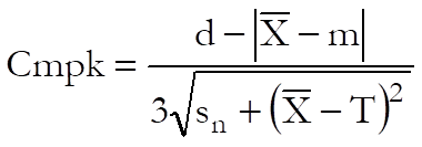
where:
![]()
![]()
![]()
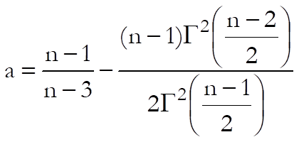
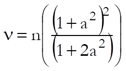
and the confidence intervals are given as:
![]()
where:
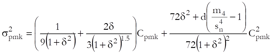
and:
![]()
Cs: Also known as Wright’s index, this index is a variation of Cpmk that performs well even when the data is skewed. Wright, P. A. (1995):
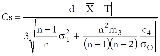
where, as before:
![]()
![]()
and c4 is the unbiasing constant.
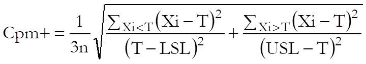
Cpm+: Boyles, R. A. (1992) proposed this index
for use when both LSL and USL are given and ![]() ,
, ![]() :
:
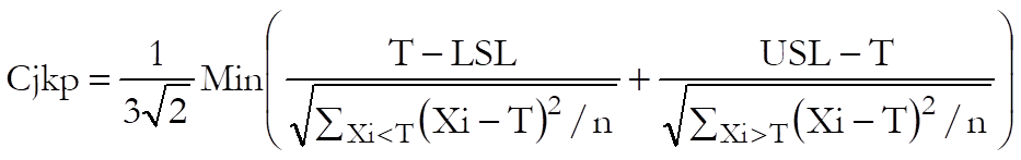
Cjkp: Also called the flexible index, this is for use when both LSL and USL are given, Kotz, S. and Johnson, N. L. (1993):
Capability Indices: Pooled Standard Deviation: If more than one data variable and / or one or more factor variables are selected, then capability indices are also calculated based on the pooled standard deviation and degrees of freedom.
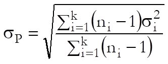
![]()
where k is the number of subgroups.
Cp, Cpl, Cpu, Cpk: These indices are calculated as above, but the pooled standard deviation and the pooled degrees of freedom are used.
Ccpk: This index is reported for subgroup analysis only. It is similar to Cpk, but is centred at the target, when a target value is provided.
When both LSL and USL are given, then:
![]()
where ![]() is
the pooled standard deviation and:
is
the pooled standard deviation and:
![]()
when a target value is given, and:
![]()
otherwise.
When LSL is given but USL is not available:
![]()
and when USL is given but LSL is not available:
![]()
In both cases,
![]()
when a target value is given, and:
![]()
otherwise.
Capability Indices: Nonparametric: The standard Process Capability Analysis assumes normal distribution of data. When this is not the case, a nonparametric (i.e. distribution-free) capability index will be useful. The methods used in computing the quantiles and their confidence limits are reported in the header. These methods can be changed using the dialogues of the Quantiles (Percentiles) procedure (see sections 5.1.3.1. Quantile Methods and 5.1.3.2. Quantile Interval Methods).
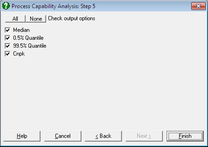
Cnpk is a variant of Cpk used for non-normal data and is defined as:
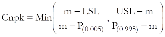
where m is the median and P(0.005) and P(0.995) are the 0.5th and 99.5th percentiles respectively.
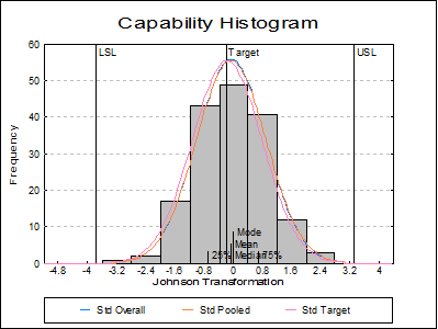
Capability Histogram: A histogram of data is displayed to help visualise its distribution. LCL, target, UCL values are indicated as well as mean median mode and quartiles (also see Histogram).
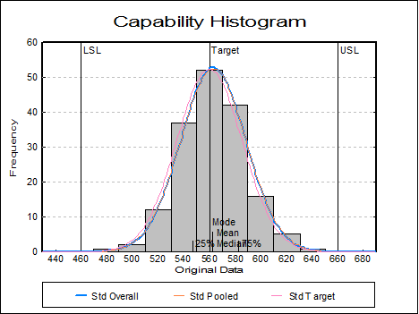
Up to six distributions can also be fitted and
displayed on the histogram. The first three of these are reserved by the
program to display normal curves with overall and pooled (if data has
subgroups) standard deviations and with deviation around the target (if a
target has been specified, see definition of ![]() above). The remaining three
distributions are set by default to Weibull, lognormal and gamma distributions,
but these can be changed by selecting Edit → Distributions dialogue from the graphics menu, after
clicking on the [Opt] button situated to the left of the Capability
Histogram check box on the Output Options Dialogue.
above). The remaining three
distributions are set by default to Weibull, lognormal and gamma distributions,
but these can be changed by selecting Edit → Distributions dialogue from the graphics menu, after
clicking on the [Opt] button situated to the left of the Capability
Histogram check box on the Output Options Dialogue.
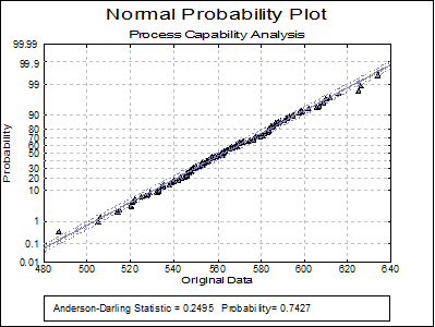
Normal Probability Plot: Original Data: A Normal Probability Plot of the original data is displayed together with Anderson-Darling Test results in the legend. You can compare this graph with the next one to visualise the improvement provided by the transformation – if there is one.
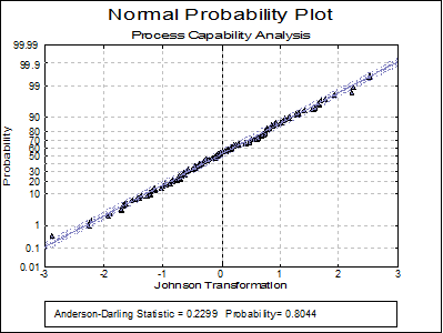
Normal Probability Plot: Transformed Data: This option is enabled if a transformation has been selected in the previous dialogue. A Normal Probability Plot of the transformed data is displayed together with Anderson-Darling Test results in the legend. You can compare this graph with the previous one to visualise the improvement provided by the transformation.
9.3.6.4. Process Capability Analysis Example
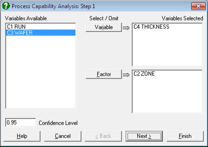
Open TIMESER and select Statistics 2 → Quality Control → Process Capability Analysis. From the Variable Selection Dialogue select THICKNESS (C21) as [Variable] and ZONE (C19) as [Factor]. On Step 2 select all levels of ZONE enter on the next dialogue 460, 560 and 660 for LSL, Target and USL respectively. Select Johnson Transformation.
Process Capability Analysis
Process Data
Variables Selected: THICKNESS
Subsample selected by: ZONE = 1, 2, 3, 4
|
Valid Cases = |
168 |
|
Number of Subgroups = |
4 |
|
Control Range = |
6.0000 |
|
Original Process Data: |
|
|
LSL = |
460.0000 |
|
Target = |
560.0000 |
|
USL = |
660.0000 |
|
Mean = |
563.0357 |
|
Overall Standard Deviation = |
25.3847 |
|
Pooled Standard Deviation = |
25.5069 |
|
Transformed Process Data: |
|
|
LSL = |
-3.7597 |
|
Target = |
-0.1694 |
|
USL = |
3.3276 |
|
Mean = |
-0.0588 |
|
Overall Standard Deviation = |
0.9600 |
|
Pooled Standard Deviation = |
0.9644 |
Data Transformation: Results
|
Z-statistic for best fit = |
0.7100 |
|
Gamma = |
-0.3867 |
|
Delta = |
4.8986 |
|
Xi = |
126.7984 |
|
Lambda = |
554.3748 |
Transformation selected: Johnson Unbounded System (SU)
z = Gamma + Delta * ASINH((x – Xi) / Lambda), Xi < x
z = -0.386691047854535 + 4.89859585514262 * ASINH((x – 554.374813248812) / 126.798395166468)
Normality Tests
Smaller probabilities indicate non-normality.
|
|
A-D Stat |
Probability |
|
Original Data |
0.2495 |
0.7427 |
|
Transformed Data |
0.2299 |
0.8044 |
Transformed Data
|
|
Original Data |
Transformed Data |
Group |
|
1 |
487.0000 |
-2.8805 |
3 |
|
2 |
505.0000 |
-2.2490 |
3 |
|
3 |
506.0000 |
-2.2130 |
4 |
|
… |
… |
… |
… |
|
166 |
625.0000 |
2.2174 |
3 |
|
167 |
626.0000 |
2.2511 |
1 |
|
168 |
634.0000 |
2.5165 |
3 |
Performance: Parts Per Million
|
|
PPM < LSL |
PPM > USL |
PPM Total |
|
Observed |
0.0000 |
0.0000 |
0.0000 |
|
Overall |
57.7873 |
209.5823 |
267.3697 |
|
Pooled |
62.1538 |
222.8973 |
285.0511 |
Performance: Percent
|
|
% < LSL |
% > USL |
% Total |
|
Observed |
0.0000 |
0.0000 |
0.0000 |
|
Overall |
0.0058 |
0.0210 |
0.0267 |
|
Pooled |
0.0062 |
0.0223 |
0.0285 |
Capability Indices: Overall Standard Deviation
|
|
Value |
Lower 95% |
Upper 95% |
|
Cp |
1.2305 |
1.0986 |
1.3623 |
|
Cpl |
1.2851 |
0.9906 |
0.9919 |
|
Cpu |
1.1759 |
0.9906 |
0.9919 |
|
Bissell Cpk |
1.1759 |
1.0401 |
1.3117 |
|
ZSW Eq 6 Cpk |
1.1759 |
1.0484 |
1.3034 |
|
ZSW Eq 8 Cpk |
1.1759 |
1.0392 |
1.3126 |
|
Chang Cpm |
1.2063 |
1.0974 |
1.3137 |
|
Boyles Cpm |
1.2099 |
1.1006 |
1.3176 |
|
SAS Cpm |
1.2224 |
1.0950 |
1.3569 |
|
NIST Cpm |
1.2224 |
1.0918 |
1.3529 |
|
Cpmk |
1.1716 |
1.0752 |
1.2680 |
|
Cs |
1.1547 |
|
|
|
Cpm+ |
0.0070 |
|
|
|
Cjkp |
1.1054 |
|
|
Capability Indices: Pooled Standard Deviation
|
|
Value |
Lower 95% |
Upper 95% |
|
Cp |
1.2248 |
1.0923 |
1.3571 |
|
Cpl |
1.2792 |
0.9906 |
0.9919 |
|
Cpu |
1.1705 |
0.9906 |
0.9919 |
|
Bissell Cpk |
1.1705 |
1.0341 |
1.3068 |
|
Ccpk |
1.2087 |
|
|
Capability Indices: Nonparametric
Quantile Method: Simple Average
Interval Method: Normal Approximation
|
|
Value |
Lower 95% |
Upper 95% |
|
Median |
-0.0730 |
-0.3239 |
0.1003 |
|
0.5% Quantile |
-2.8805 |
* |
-1.9213 |
|
99.5% Quantile |
2.5165 |
1.9091 |
* |
|
Cnpk |
1.3132 |
|
|