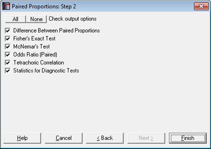
6.4.5. Paired Proportions
A 2 x 2 table is formed to perform procedures in this section. The data can be in the form of two binary factors or two continuous variables split into two groups by two cutpoints. It is also possible to enter directly the four cell frequencies as explained at the beginning of this chapter (see 6.0.7. 2 x 2 Tables). The user should take care to distinguish this table from a table formed on the same pair of columns by the Unpaired Proportions procedure. Here, the total table frequency is the number valid pairs (as in 2 x 2 cross-tabulation), whereas in Unpaired Proportions the total frequency is the sum of valid cases in sample 1 and sample 2.
The two columns usually contain measurements on the same sample before and after a certain treatment.
When the four frequency values for a 2 x 2 table are already available in the spreadsheet, you do not have to type them again into the Cell Frequencies are Given dialogue. All statistics available under Binomial Proportion, Unpaired Proportions and Paired Proportions procedures are also available in Contingency Table and Cross-Tabulation procedures (see 6.6.2.3. 2 x 2 Table Statistics).
6.4.5.1. Difference Between Paired Proportions
As in the previous section, the null hypothesis “the two proportions are equal” is tested (see 6.4.4.1. Difference Between Unpaired Proportions). That is:
![]()
where:
![]() ,
, ![]()
See Gardner & Altman (2000) p. 52, the traditional method. The test statistic based on normal approximation is defined as:
![]()
with a standard error of:
![]()
The asymptotic confidence limits are computed as:
![]()
The exact probability is determined using the binomial distribution and the exact confidence limits are based on the definitions introduced for the Binomial Test:
![]()
![]()
Example 1
Example 4.9 on p. 123 from Armitage & Berry (2002). Distribution of sputum according to results of culture on two media are given in the form of a 2 x 2 table.
Select Statistics 1 → Nonparametric Tests (1-2 Samples) → Paired Proportions and select the data option 3 Cell Frequencies are Given. Enter 20 in (1,1), 12 in (1,2), 2 in (2,1), 16 in (2,2) and check only the Difference Between Paired Proportions output option to obtain the following results:
Paired Proportions
Data option: Cell Frequencies are Given
|
|
1 |
2 |
Total |
|
1 |
20 |
2 |
22 |
|
2 |
12 |
16 |
28 |
|
Total |
32 |
18 |
50 |
Difference Between Paired Proportions
|
Proportion 1 = |
0.0400 |
|
Proportion 2 = |
0.2400 |
|
|
Difference |
2-Tail Probability |
Lower 95% |
Upper 95% |
|
Asymptotic |
-0.2000 |
0.0075 |
-0.3358 |
-0.0642 |
|
Exact Binomial |
|
0.0129 |
0.0402 |
0.2700 |
Example 2
Example on p. 32, Gardner & Altman (1989). Inadequacy of monitoring in hospital of deaths and survivors among asthma patients is given in the form of a 2 x 2 table.
Select Statistics 1 → Nonparametric Tests (1-2 Samples) → Paired Proportions and select the data option 3 Cell Frequencies are Given. Enter 10 in (1,1), 3 in (1,2), 13 in (2,1), 9 in (2,2) and check only the Difference Between Paired Proportions output option to obtain the following results:
Paired Proportions
Data option: Cell Frequencies are Given
|
|
1 |
2 |
Total |
|
1 |
10 |
13 |
23 |
|
2 |
3 |
9 |
12 |
|
Total |
13 |
22 |
35 |
Difference Between Paired Proportions
|
Proportion 1 = |
0.3714 |
|
Proportion 2 = |
0.0857 |
|
|
Difference |
Standard Error |
Z-Statistic |
1-Tail Probability |
2-Tail Probability |
|
Asymptotic |
0.2857 |
0.1036 |
2.5000 |
0.0062 |
0.0124 |
|
Exact Binomial |
|
|
|
0.0106 |
0.0213 |
|
|
Lower 95% |
Upper 95% |
|
Asymptotic |
0.0827 |
0.4887 |
|
Exact Binomial |
0.0398 |
0.4201 |
6.4.5.2. Fisher’s Exact Test
Under the assumption of independence of column and row factors, the probability of the observed 2 x 2 table (the table probability) follows the hypergeometric distribution:
![]()
where nij are the cell frequencies and:
![]()
![]()
![]()
The following four probabilities are reported.
Right-Tail Probability: Sum of all possible table probabilities with the same observed row and column totals where n11 is greater than or equal to the observed n11. Use this to test positive association between the two factors.
Left-Tail Probability: Sum of all possible table probabilities with the same observed row and column totals where n11 is less than or equal to the observed n11. Use this to test negative association between the two factors.
2-Tail Probability: Sum of all table probabilities with the same observed row and column totals. Use this to test association between the two factors.
Table Probability: The probability of the observed table PT as defined above.
You can perform Fisher’s Exact Test for R x C Tables (i.e. tables larger than 2 x 2), using the Cross-Tabulation procedure (see 6.6.2.2.2. Fisher’s Exact Test).
Example
Example 24.22 on p. 568 from Zar, J. H. (2010). Data is given in the form of 2 x 2 contingency tables.
Paired Proportions
Data option: Cell Frequencies are Given
|
|
1 |
2 |
Total |
|
1 |
12 |
7 |
19 |
|
2 |
2 |
9 |
11 |
|
Total |
14 |
16 |
30 |
Fisher’s Exact Test
|
|
Left-Tail Probability |
Right-Tail Probability |
Two-Tail Probability |
Table Probability |
|
Fisher’s Exact |
0.99787 |
0.02119 |
0.02589 |
0.01906 |
Zar reports the right-tail and two-tailed probabilities.
6.4.5.3. McNemar Test
McNemar is a chi-square statistic used to test whether the first row and first column totals are equal.
Asymptotic without Continuity Correction: The chi-square statistic is:
![]()
![]()
Asymptotic with Continuity Correction:
![]()
![]()
Exact Binomial: The exact probability is calculated from the binomial function:
![]()
and the exact confidence limits are given by Liddell (1983) as:
![]()
![]()
Example
Example 24.17 on p. 571 from Zar, J. H. (2010). Data is recorded in the form of a 2 x 2 contingency table. The null hypothesis “the proportion of persons experiencing relief is the same with both locations” is tested.
|
|
|
Lotion 1 |
|
|
|
|
Relief |
No relief |
|
Lotion 2 |
Relief |
12 |
5 |
|
|
No relief |
11 |
22 |
Select Statistics 1 → Nonparametric Tests (1-2 Samples) → Paired Proportions and select the data option 3 Cell Frequencies are Given. Enter 12 in (1,1), 11 in (1,2), 5 in (2,1), 22 in (2,2). Next, select only the McNemar Test option.
Paired Proportions
Data option: Cell Frequencies are Given
|
|
1 |
2 |
Total |
|
1 |
12 |
5 |
17 |
|
2 |
11 |
22 |
33 |
|
Total |
23 |
27 |
50 |
McNemar’s Test
|
|
Chi-Square Statistic |
Degrees of Freedom |
Right-Tail Probability |
|
Asymptotic |
2.2500 |
1 |
0.1336 |
|
Asymptotic with CC |
1.5625 |
1 |
0.2113 |
|
|
2-Tail Probability |
Lower 95% |
Upper 95% |
|
Exact Binomial |
1.0000 |
0.7047 |
8.0769 |
Since p > 0.05 do not reject the null hypothesis.
6.4.5.4. Odds Ratio (Paired)
The odds ratio for paired cases is computed as:
![]()
The exact confidence limits are based on the definitions introduced for the Binomial Test:
![]()
![]()
For the odds ratio for unpaired cases see 6.4.4.3. Odds Ratio and Relative Risks.
Example
Example on p. 66, Gardner Altman (2000). Inadequacy of monitoring in hospital of deaths and survivors among asthma patients is given in the form of a 2 x 2 table.
Select Statistics 1 → Nonparametric Tests (1-2 Samples) → Paired Proportions and select the data option 3 Cell Frequencies are Given. Enter 10 in (1,1), 3 in (1,2), 13 in (2,1), 9 in (2,2) and check only the Odds Ratio (Paired) output option:
Paired Proportions
Data option: Cell Frequencies are Given
|
|
1 |
2 |
Total |
|
1 |
10 |
13 |
23 |
|
2 |
3 |
9 |
12 |
|
Total |
13 |
22 |
35 |
Odds Ratio (Paired)
|
|
Value |
Lower 95% |
Upper 95% |
|
Odds Ratio (Paired) |
4.3333 |
1.1908 |
23.7074 |
6.4.5.5. Tetrachoric Correlation
The Tetrachoric Correlation coefficient is computed as follows:
![]()
where:
![]()
is the tetrachoric ratio.
Example
Table 58 on p. 167 from Cohen, L. & M. Holliday (1983). The raw data is not available on individual success ratings, but a 2 x 2 contingency table is given on satisfactory / unsatisfactory ratings on a basic computing course.
|
Frequency (1,1) |
40 |
|
Frequency (1,2) |
10 |
|
Frequency (2,1) |
20 |
|
Frequency (2,2) |
30 |
Select Statistics 1 → Nonparametric Tests (1-2 Samples) → Paired Proportions → Tetrachoric Correlation, select the data option Cell Frequencies are Given and enter the values as given in the above table to obtain the following results:
Paired Proportions
Data option: Cell Frequencies are Given
|
|
1 |
2 |
Total |
|
1 |
40 |
10 |
50 |
|
2 |
20 |
30 |
50 |
|
Total |
60 |
40 |
100 |
Tetrachoric Correlation
|
|
Ratio |
Tetrachoric Correlation |
|
|
6.0000 |
0.6132 |
6.4.5.6. Statistics for Diagnostic Tests
Define the 2 x 2 table entries as follows:
|
|
Positive Actual |
Negative Actual |
Total |
|
Positive Estimate |
TP |
FP |
TP + FP |
|
Negative Estimate |
FN |
TN |
FN + TN |
|
Total |
TP + FN |
FP + TN |
TOTAL |
where:
TP: True Positive: Correct acceptance,
TN: True Negative: Correct rejection,
FP: False Positive: False alarm (Type I error),
FN: False Negative: Missed detection (Type II error).
There are two important points we need to emphasize here to ensure that the 2 x 2 table generated by the Paired Proportions procedure conforms to these definitions. First, you need to select the factor representing the Actual state as Column 1 from the Variable Selection Dialogue so that it appears at the top of the table. Secondly, as the Paired Proportions procedure sorts the factor levels in ascending order, the smaller values of the two factors selected are assumed to represent the positive outcome. If the larger values represent the positive outcome in your data, you will need to recode your factor columns first, so that the smaller values represent the positive outcome. Otherwise the statistics below will not be computed correctly.
Many of the statistics displayed here are proportions and their confidence intervals are computed employing the Wald (asymptotic) and Clopper-Pearson (exact) methods for binomial proportions (see 6.4.3.2. Binomial Test). Confidence intervals for likelihood ratios are computed as in Simel D., Samsa G., Matchar D. (1991).
Sensitivity: True positive rate or the probability of diagnosing a case as positive when it is actually positive.
TP / (TP + FN)
Specificity: True negative rate or the probability of diagnosing a case as negative when it is actually negative.
TN / (TN + FP)
Accuracy: The rate of correctly classified or the probability of true positive results, including true positive and true negative.
Sensitivity * Prevalence + Specificity * (1 – Prevalence)
(TP + TN) / TOTAL
Prevalence: The actual positive rate.
(TP + FN) / TOTAL
Apparent Prevalence: The estimated positive rate.
(TP + FP) / TOTAL
Youden’s Index: Confidence intervals are calculated as in Bangdiwala S.I., Haedo A.S., Natal M.L. (2008).
Sensitivity + Specificity
TP / (TP + FN) + TN / (FP + TN)
Positive Predictive Value: PPV
TP / (TP + FP)
Negative Predictive Value: NPV
TN / (FN + TN)
Positive Likelihood Ratio: LR+
Sensitivity / (1 – Specificity)
(TP / (TP + FN)) / (1 – (TN / (FP + TN)))
Negative Likelihood Ratio: LR-
(1 – Sensitivity) / Specificity
(1 – (TP / (TP + FN))) / (TN / (FP + TN))
Diagnostic Odds Ratio: Confidence intervals are calculated as in Scott I.A., Greenburg P.B., Poole P.J. (2008).
Positive Likelihood Ratio / Negative Likelihood Ratio
(TP * TN) / (FP * FN)
Weighted Positive Likelihood Ratio: WLR+. LR+ is weighted by prevalence.
(Prevalence * Sensitivity) / ((1-Prevalence)(1-Specificity))
TP / FP
Weighted Negative Likelihood Ratio: WLR-. LR- is weighted by prevalence.
(Prevalence (1-Sensitivity)) / ((1-Prevalence) Specificity)
FN / TN
Example
Table 19.47, Case (b) on p. 694 from Armitage & Berry (2002). The data is available as a 2 x 2 contingency table:
|
Frequency (1,1) |
90 |
|
Frequency (1,2) |
90 |
|
Frequency (2,1) |
10 |
|
Frequency (2,2) |
810 |
Select Statistics 1 → Nonparametric Tests (1-2 Samples) → Paired Proportions → Statistics for Diagnostic Tests, select the data option Cell Frequencies are Given and enter the values as given in the above table to obtain the following results:
Paired Proportions
Data option: Cell Frequencies are Given
|
|
1 |
2 |
Total |
|
1 |
90 |
90 |
180 |
|
2 |
10 |
810 |
820 |
|
Total |
100 |
900 |
1000 |
Statistics for Diagnostic Tests
Smaller factor level represents the positive outcome.
Confidence Intervals: Row 1: Asymptotic Normal, Row 2: Exact Binomial
|
|
Value |
Standard Error |
Lower 95% |
Upper 95% |
|
Sensitivity |
0.9000 |
0.0300 |
0.8412 |
0.9588 |
|
|
|
|
0.8238 |
0.9510 |
|
Specificity |
0.9000 |
0.0100 |
0.8804 |
0.9196 |
|
|
|
|
0.8785 |
0.9188 |
|
Accuracy |
0.9000 |
0.0095 |
0.8814 |
0.9186 |
|
|
|
|
0.8797 |
0.9179 |
|
Prevalence |
0.1000 |
0.0095 |
0.0814 |
0.1186 |
|
|
|
|
0.0821 |
0.1203 |
|
Apparent Prevalence |
0.1800 |
0.0121 |
0.1562 |
0.2038 |
|
|
|
|
0.1567 |
0.2052 |
|
Youden’s Index |
0.8000 |
|
|
|
|
|
|
|
0.7023 |
0.8698 |
|
Positive Predictive Value |
0.5000 |
0.0373 |
0.4270 |
0.5730 |
|
|
|
|
0.4247 |
0.5753 |
|
Negative Predictive Value |
0.9878 |
0.0038 |
0.9803 |
0.9953 |
|
|
|
|
0.9777 |
0.9941 |
|
Positive Likelihood Ratio |
9.0000 |
|
7.3201 |
11.0654 |
|
Negative Likelihood Ratio |
0.1111 |
|
0.0617 |
0.2001 |
|
Diagnostic Odds Ratio |
81.0000 |
|
40.6821 |
161.2749 |
|
Weighted Positive Likelihood Ratio |
1.0000 |
|
0.8133 |
1.2295 |
|
Weighted Negative Likelihood Ratio |
0.0123 |
|
0.0067 |
0.0229 |