9.5.2. Inverse Fourier Transform
The real and imaginary parts of the series in the time domain is displayed.
Example
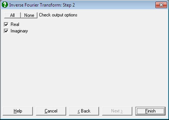
Carry out the example in Fourier Transform above. If you are using UNISTAT in Stand-Alone Mode, click on the UNISTAT icon on the Output Medium Toolbar to send the output table to UNISTAT spreadsheet. In Excel Add-In Mode select the output matrix as data. Then select Statistics 2 → Fourier Analysis → Inverse Fourier Transform. From the Variable Selection Dialogue select Real (C17) as [Real] and Imaginary (C18) as [Imaginary]to obtain the following results:
Inverse Fourier Transform
Real: Real, Imaginary: Imaginary
|
|
Real |
Imaginary |
|
1 |
95.7300 |
0.0000 |
|
2 |
94.5200 |
-0.0000 |
|
3 |
93.2900 |
-0.0000 |
|
4 |
96.9200 |
-0.0000 |
|
5 |
88.8900 |
-0.0000 |
|
6 |
98.1600 |
-0.0000 |
|
7 |
97.0300 |
-0.0000 |
|
8 |
100.3100 |
-0.0000 |
|
9 |
102.1200 |
0.0000 |
|
10 |
102.4800 |
-0.0000 |
|
11 |
102.3100 |
-0.0000 |
|
12 |
102.5900 |
0.0000 |
|
13 |
83.3500 |
-0.0000 |
|
14 |
94.6100 |
0.0000 |
|
15 |
96.5000 |
0.0000 |
|
16 |
93.6900 |
0.0000 |
|
17 |
84.7600 |
0.0000 |
|
18 |
88.0200 |
0.0000 |
|
19 |
83.7300 |
0.0000 |
|
… |
… |
… |
|
50 |
61.7400 |
-0.0000 |
|
51 |
61.7600 |
0.0000 |
|
52 |
61.6100 |
0.0000 |
|
53 |
71.4700 |
-0.0000 |
|
54 |
66.7900 |
-0.0000 |
|
55 |
69.0800 |
-0.0000 |
|
56 |
68.3500 |
-0.0000 |
|
57 |
72.5300 |
-0.0000 |
|
58 |
65.7400 |
-0.0000 |
|
59 |
84.5066 |
0.0000 |
|
60 |
84.5066 |
-0.0000 |
|
61 |
84.5066 |
0.0000 |
|
62 |
84.5066 |
-0.0000 |
|
63 |
84.5066 |
-0.0000 |
|
64 |
84.5066 |
-0.0000 |
We can see that the real part is the same as Interest (C4) with the mean value added in rows 59 to 64. The imaginary part is almost zero, except for the accumulated round-off errors.