6.7.1. One Sample

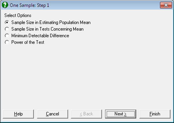
The first procedure provided here concerns estimation of population mean and as such it is inherently different from the last three, which are derived from the same equation, each time solving for a different parameter.

6.7.1.1. Sample Size in Estimating the Population Mean

The sample size necessary to achieve the desired level of precision in estimating a population mean is given by the following formula:

  

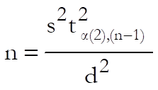
Here:

·      s² is the sample variance with ν degrees of freedom,

·      d is the half-width of the desired confidence interval,

·      1 - α is the confidence level,

·      1 - β is the assurance that the confidence interval will not be greater,

·      is the two-tailed critical value for α from t-distribution with (n - 1) degrees of freedom.

Since critical value of t on the right hand side of this equation depends on the sample size n, the left hand side cannot be computed directly. Therefore, an iterational convergence algorithm is employed.

The user is expected to enter:

·      Denominator Degrees of Freedom

·      Sample Variance

·      Half-Width of Confidence Interval

·      Assurance for Confidence Interval

·      Confidence Level

and the program will output the estimated sample size.

Example

Example 7.7 on p. 115 from Zar, J. H. (2010). Select Statistics 1 → Sample Size and Power Estimation → One Sample and the Sample Size in Estimating Population Mean option. Enter the following data at the next dialogue to obtain the Estimated Sample Size:

Sample Size and Power Estimation: One Sample

Sample Size in Estimating Population Mean

 

Denominator Degrees of Freedom =	2.0000
Sample Variance =	0.4008
Half-Width of Confidence Interval =	0.2500
Assurance for Confidence Interval =	0.9000
Confidence Level =	0.9500
Estimated Sample Size =	27.0740

 

6.7.1.2. Sample Size in Tests Concerning the Mean

The purpose of the experiment is to test if the sample is taken from a population with a specified mean “H₀: μ = μ₀” or it is from a population with a different mean “H₀: μ  μ₀”.

Sample size in tests about the mean is determined from:

  

Here:

·      s² is the sample variance with ν degrees of freedom,

·      δ is the minimum detectable difference between the two population means at the desired confidence interval,

·      α is the probability of committing a Type I error and 1- α is the confidence level, which can be one or two-tailed.

·      β is the probability of committing a Type II error and 1 - β is the power of the test,

·      is the (one or) two-tailed critical value for α from t-distribution with ν degrees of freedom,

·       is the one-tailed critical value for β from t-distribution with ν degrees of freedom.

Since critical values of t on the right hand side of this equation are dependent on the sample size n, an iterational algorithm is employed.

The user is expected to enter:

·      Sample Variance

·      Minimum detectable difference

·      Power of the test

·      Confidence Level

·      1 or 2 tailed test

and the program will output the estimated sample size.

Example

Example 7.8 on p. 116 from Zar, J. H. (2010). Select Statistics 1 → Sample Size and Power Estimation → One Sample and the Sample Size in Tests Concerning Mean option. Enter the following data at the next dialogue to obtain the Estimated Sample Size:

Sample Size and Power Estimation: One Sample

Sample Size in Tests Concerning Mean

Sample Variance =	1.5682
Minimum Detectable Difference =	1.0000
Power of the Test =	0.9000
Confidence Level =	0.9500
1 or 2 Tailed Test =	2.0000
Estimated Sample Size =	18.4991

 

6.7.1.3. Minimum Detectable Difference for One Sample

Rearranging the equation in section 6.7.1.2. Sample Size in Tests Concerning the Mean we obtain:

  

Here, δ can be computed directly, without an iterational algorithm, as all parameters on the right hand side can be computed using the given parameters.

The user is expected to enter:

·      Sample Size

·      Sample Variance

·      Power of the test

·      Confidence Level

·      1 or 2 tailed test

and the program will output the minimum detectable difference.

Example

Example 7.9 on p. 117 from Zar, J. H. (2010). Select Statistics 1 → Sample Size and Power Estimation → One Sample and the Minimum Detectable Difference option. Enter the following data at the next dialogue:

Sample Size and Power Estimation: One Sample

Minimum Detectable Difference

Sample Size =	25.0000
Sample Variance =	1.5682
Power of the Test =	0.9000
Confidence Level =	0.9500
1 or 2 Tailed Test =	2.0000
Minimum Detectable Difference =	0.8470

 

6.7.1.4. Power of the Test for One Sample

Rearranging the equation in section 6.7.1.2. Sample Size in Tests Concerning the Mean we obtain:

  

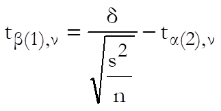
Here,  can be computed directly, as all parameters on the right hand side can be computed using the given parameters. Then β is obtained from t-distribution with ν degrees of freedom.

The user is expected to enter:

·      Sample Size

·      Sample Variance

·      Minimum Detectable Difference

·      Confidence Level

·      1 or 2 tailed test

and the program will output the t-statistic and its p-value.

Example

Example 7.10 on p. 118 from Zar, J. H. (2010). Select Statistics 1 → Sample Size and Power Estimation → One Sample and the Power of the Test option. Enter the following data at the next dialogue:

Sample Size and Power Estimation: One Sample

Power of the Test

Sample Size =	12.0000
Sample Variance =	1.5682
Minimum Detectable Difference =	1.0000
Confidence Level =	0.9500
1 or 2 Tailed Test =	2.0000
Power of the Test:
t-Statistic =	0.9480
2-Tail Probability =	0.8204