8.4. Principal Components Analysis
This is the core multivariate analysis procedure. All other multivariate methods (except for Cluster Analysis) can be considered as variations of Principal Components Analysis (PCA). The basic idea behind PCA is to redraw the axis system for n dimensional data such that points lie as close as possible to the axes. The derived variables, also called principal components, can express a large proportion of total variance of the data with a smaller number of variables.
From a mathematical point of view, the problem of PCA consists of finding eigenvectors of the standardised or non standardised sum of squared products (SSP) matrix for the raw data. The standard and non standard SSP matrices are directly proportional to simple correlations and covariance matrices for the same data respectively.
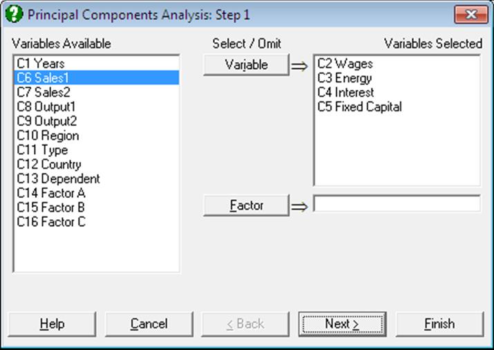
Select raw data columns to analyse by clicking on [Variable]. There is also an optional [Factor] button available to run predictions.
Predictions: The rows of the factor column containing a missing value will not be included in calculations. However, if no other variable contains a missing value, then the PCA transformation will be applied to them. They will be indicated in all plots by an @ character and in case-wise tables by an asterisk (*). In this way, it is possible to obtain transformations on a set of observed cases and simultaneously apply the transformation to a number of test cases.
It is possible to use markers other than missing data to designate cases as test cases. Suppose, for instance, you wish the program to interpret cases with -1 in their group variable as test cases. To do this, enter the following line in the [Options] section of Documents\Unistat10\Unistat10.ini file:
DiscrPredict=-1
8.4.1. Principal Components Output Options
The following output options are available:
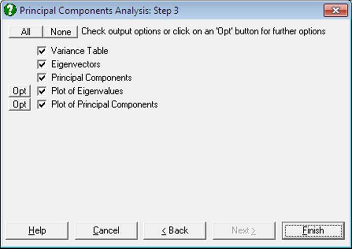
Variance Table: Eigenvalues are scaled such that their total variance is equal to the total number of variables. It is often concluded that a principle component with an eigenvalue greater than one makes a significant contribution to the total variance.
Eigenvectors: These are the coefficients which transform original data into the new coordinates. Each eigenvector is scaled such that the sum of squares of its elements is unity.
Principal Components: These are the transformed variables obtained by multiplying the original data matrix with the matrix of eigenvectors. When the analysis is carried out on a correlation or covariance matrix, the Principal Components table and plot options will not be available.
The Principal Components have the following properties:
1) They are uncorrelated. The Pearson’s correlation between any two Principal Components is zero.
2) Their variances are equal to their corresponding eigenvalues.
3) They are sorted in decreasing order according to their variances.
Therefore, you may examine the Variance Table (the eigenvalues), decide on the first r eigenvalues according to the percentage of variation you want to retain, then save the Principal Components to data and then retain only those first r Principal Components for further analysis.
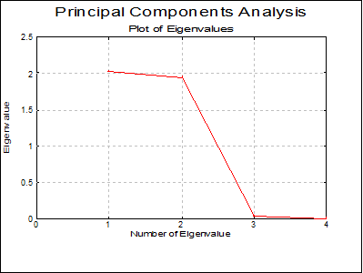
Plot of Eigenvalues (Scree Plot): This is also called the scree plot. Eigenvalues and their corresponding eigenvectors are sorted in decreasing order. Typically, this plot will fall sharply with the first few eigenvalues and then get less and less steep.
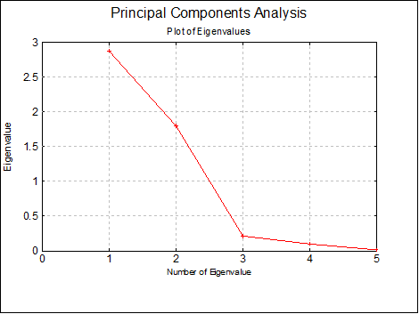
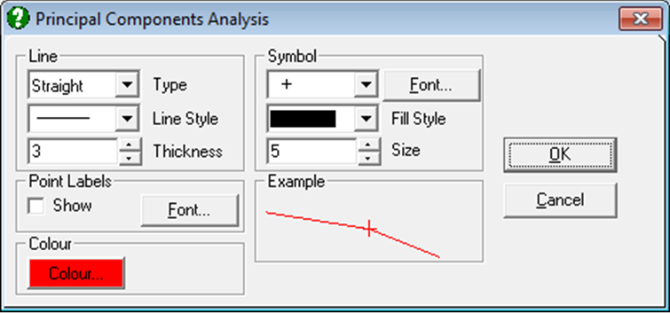
You can edit properties of the graph by selecting Edit → XY Points from the menu.
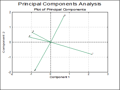
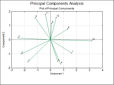
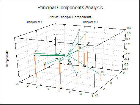
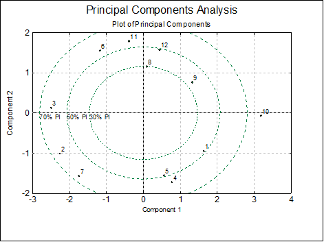
Plot of Principal Components: This is the plot of transformed variables displayed in the Principal Components table. First, a dialog allows you to choose which components to be plotted.
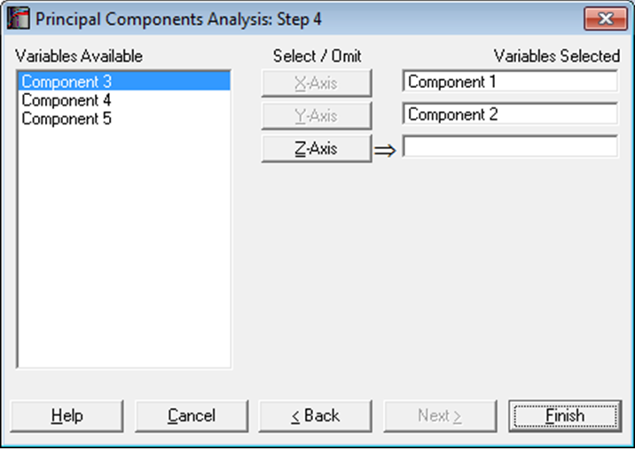
The program will display a 2D graph if you select two variables to plot,
and a 3D graph if you select three variables.
The Edit → XY Points menu option can be used to edit the graph properties.
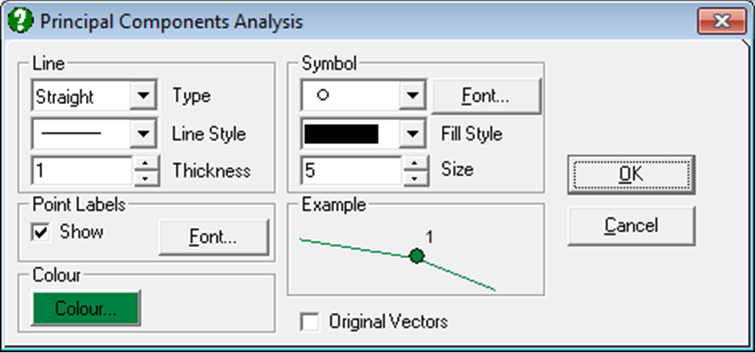
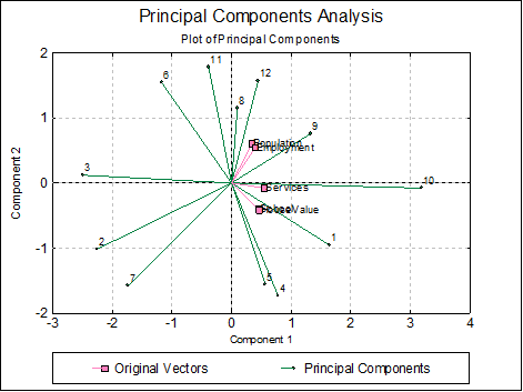
By checking the Original Vectors box, the original variables can be plotted alongside the transformed data points.
If you select the Ellipse option from the Line Type list, a further dialogue will pop up allowing you to draw interval ellipses for the mean of Y (confidence) and / or actual Y (prediction) values at one or more confidence levels.
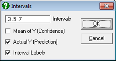
Either or both intervals or none can be drawn by checking the boxes as desired. The text box can be used to enter multiple confidence levels between 0 and 1, separated by spaces. When the last box is checked, a label will be printed for each interval curve. For further details see Ellipse For further details see Ellipse Confidence and Prediction Intervals in 4.1.1.1.1. Line.
8.4.2. Principal Components Example
Table 12.2 on p. 607. Tabachnick, B. G. & L. S. Fidell (1989).
Open MULTIVAR, select Statistics 2 → Principal Components Analysis and select Cost, Lift, Depth, Powder (C6 to C9) as [Variable]s. Select Output and All to obtain the following results:
Principal Components Analysis
Variance Table
|
Component No |
Eigenvalue |
Cumulative Variance |
Percent |
Cumulative |
|
1 |
2.0163 |
2.0163 |
0.5041 |
0.5041 |
|
2 |
1.9415 |
3.9578 |
0.4854 |
0.9895 |
|
3 |
0.0378 |
3.9956 |
0.0095 |
0.9989 |
|
4 |
0.0044 |
4.0000 |
0.0011 |
1.0000 |
Eigenvectors
|
|
Dimension 1 |
Dimension 2 |
Dimension 3 |
Dimension 4 |
|
Cost |
-0.3524 |
0.6143 |
0.6625 |
0.2439 |
|
Lift |
0.2511 |
-0.6638 |
0.6759 |
0.1988 |
|
Depth |
0.6274 |
0.3222 |
0.2755 |
-0.6532 |
|
Powder |
0.6474 |
0.2796 |
-0.1685 |
0.6887 |
Principal Components
|
|
Dimension 1 |
Dimension 2 |
Dimension 3 |
Dimension 4 |
|
1 |
2.1766 |
-0.8161 |
0.0820 |
-0.0379 |
|
2 |
0.7102 |
1.7180 |
-0.1123 |
0.0692 |
|
3 |
-0.9445 |
0.6479 |
-0.1456 |
-0.0930 |
|
4 |
-0.8213 |
-1.8991 |
-0.1302 |
0.0494 |
|
5 |
-1.1210 |
0.3494 |
0.3062 |
0.0123 |