6.5.1. Kruskal-Wallis One-Way ANOVA
Data entry is in multisample format (see 6.0.4. Multisample Tests). Each sample can be entered in a separate column (not necessarily of equal length), or they can be stacked in one or more columns and subsamples defined by an unlimited number of factor columns. Missing values are omitted by case.
6.5.1.1. Kruskal-Wallis ANOVA Test Results
This test is used to evaluate the degree of association between samples. It is assumed that the samples have similar distributions and that they are independent. All cases in all samples are ranked together and then the rank sum of each sample is found. The test statistic is calculated as follows:
![]()
![]()
where N is the total number of cases in all samples, M is the number of variables and R is the total of the squared sum of ranks for each sample divided by the respective sample size.
The test statistic corrected for ties is:
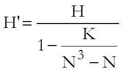
where K is sum of k3 – k and k is the number of tied cases for a particular rank.
The one-tail probability is reported from the chi-square distribution.
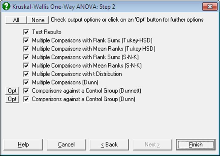
6.5.1.2. Kruskal-Wallis ANOVA Multiple Comparisons
Eight nonparametric Multiple Comparisons can be performed as part of this procedure. The last two are comparisons against a control group (which require further inputs) and the rest are comparisons between all possible pairs.
Multiple comparisons with rank sums (Tukey-HSD)
Nonparametric Multiple Comparisons are performed in a way similar to the Tukey-HSD test using rank sums. The standard error is computed as:
![]()
This test requires equal group sizes.
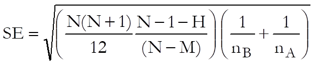
Multiple comparisons with mean ranks (Tukey-HSD)
Nonparametric Multiple Comparisons are performed in a way similar to the Tukey-HSD test using mean ranks. In this case the standard error is computed as:
![]()
This test requires equal group sizes.
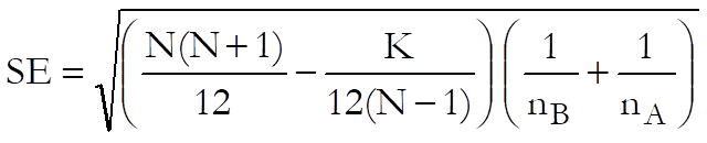
Multiple comparisons with rank sums (S-N-K)
Nonparametric Multiple Comparisons are performed in a way similar to the Student-Newman-Keuls test using mean ranks. In this case the standard error is computed as:
![]()
This test requires equal group sizes.
Multiple comparisons with mean ranks (S-N-K)
Nonparametric Multiple Comparisons can also be performed in a way similar to the Student-Newman-Keuls test using rank sums. The standard error is computed as follows:
![]()
This test requires equal group sizes.
Multiple comparisons with t-distribution
If group sizes are not equal and all possible pairs are to be compared then this option can be selected. Nonparametric Multiple Comparisons are performed in a way similar to the Tukey-HSD test using mean ranks. In this case the standard error is computed as:
Multiple comparisons (Dunn)
If group sizes are not equal and all possible pairs are to be compared, then this option can be selected.
The standard error, which has a correction term for tied ranks, is computed as follows:
where N is the total number of cases, K is the sum of k3 – k and k is the number of tied cases for a particular rank (as in Kruskal-Wallis One-Way ANOVA). In comparisons group mean ranks are used.
Comparisons against a control group (Dunnett)
If each group of data is to be tested against a control group and all groups are of the same size then select this option. If the group sizes are not equal then the next option (Dunn’s test) should be used.
The standard error is computed as follows:
![]()
The only other difference between the Dunnett test introduced here and the Dunnett test per se is that here the group rank sums are used while the latter uses group mean ranks.
Comparisons against a control group (Dunn)
If each group of data is to be tested against a control group and all groups are not of the same size then select this option. If the group sizes are equal then the previous option (Dunnett test) may also be employed.
The standard error, which has a correction term for tied ranks, is computed as in the Dunn’s test above.
6.5.1.3. Kruskal-Wallis ANOVA Examples
Example 1
Example 10.6 on p. 287 from Armitage & Berry (2002). Counts of adult worms in four groups of rats are given. The null hypothesis “there is no significant difference between the rats” is tested.
Open NONPARM1 and select Statistics 1 → Nonparametric Tests (Multisample) → Kruskal-Wallis ANOVA. Select Group 1, Group 2, Group 3 and Group 4 (C1 to C4) as [Variable]s and then select only Test Results to obtain the following results:
Kruskal-Wallis One-Way ANOVA
|
|
Cases |
Rank Sum |
Mean Rank |
|
Group 1 |
5 |
42.0000 |
8.4000 |
|
Group 2 |
5 |
53.0000 |
10.6000 |
|
Group 3 |
5 |
36.0000 |
7.2000 |
|
Group 4 |
5 |
79.0000 |
15.8000 |
|
Total |
20 |
210.0000 |
10.5000 |
|
Correction for Ties = |
0.0008 |
|
Chi-Square Statistic = |
6.2047 |
|
Degrees of Freedom = |
3 |
|
Right-Tail Probability = |
0.10207 |
This result is not significant at the 10% level. Hence do not reject the null hypothesis.
Example 2
Examples 10.10 on p. 216 and 11.7 on p. 241 from Zar, J. H. (2010). A researcher wants to test the null hypothesis “the abundance of the flies is the same in all three vegetation layers” at a 95% significance level. If they were found to be different, then the researcher would also like to know which ones.
Open NONPARM1, select Statistics 1 → Nonparametric Tests (Multisample) → Kruskal-Wallis ANOVA and include Herbs (C5), Shrubs (C6) and Trees (C7) in the analysis by clicking [Variable]. Check only the Test Results and the Multiple Comparisons with Rank Sums (Tukey-HSD) boxes to obtain the following results:
Kruskal-Wallis One-Way ANOVA
|
|
Cases |
Rank Sum |
Mean Rank |
|
Herbs |
5 |
64.0000 |
12.8000 |
|
Shrubs |
5 |
30.0000 |
6.0000 |
|
Trees |
5 |
26.0000 |
5.2000 |
|
Total |
15 |
120.0000 |
8.0000 |
|
Correction for Ties = |
0.0000 |
|
Chi-Square Statistic = |
8.7200 |
|
Degrees of Freedom = |
2 |
|
Right-Tail Probability = |
0.0128 |
Since the right tail probability is less than 5%, the null hypothesis is rejected. Next the researcher would like to find which vegetation layers have different abundance of the flies.
Multiple Comparisons with Rank Sums (Tukey-HSD)
Method: 95% Tukey-HSD interval.
** denotes significantly different pairs. Vertical bars show homogeneous subsets.
A pairwise test result is significant if its q stat value is greater than the table q.
|
Group |
Cases |
Rank Sum |
Trees |
Shrubs |
Herbs |
|
|
Trees |
5 |
26.0000 |
|
|
** |
| |
|
Shrubs |
5 |
30.0000 |
|
|
** |
| |
|
Herbs |
5 |
64.0000 |
** |
** |
|
| |
|
Comparison |
Difference |
Standard Error |
q Stat |
Table q |
Probability |
|
Herbs – Trees |
38.0000 |
10.0000 |
3.8000 |
3.3145 |
0.0197 |
|
Shrubs – Trees |
4.0000 |
10.0000 |
0.4000 |
3.3145 |
0.9569 |
|
Herbs – Shrubs |
34.0000 |
10.0000 |
3.4000 |
3.3145 |
0.0428 |
|
Comparison |
Lower 95% |
Upper 95% |
Result |
|
Herbs – Trees |
4.8551 |
71.1449 |
** |
|
Shrubs – Trees |
-29.1449 |
37.1449 |
|
|
Herbs – Shrubs |
0.8551 |
67.1449 |
** |
|
Homogeneous Subsets: |
|
|
Group 1: |
Trees Shrubs |
|
Group 2: |
Herbs |
The overall conclusion is that fly abundance is the same for Trees and Shrubs but it is different for Herbs.
Example 3
Examples 10.11 on p. 217 and 11.8 on p. 242 from Zar, J. H. (2010). The null hypothesis that “pH is the same in all four ponds” is tested at a 95% significance level. If they were found to be different, then we would also like to know which ones. The data has unequal column lengths.
Open NONPARM1, select Statistics 1 → Nonparametric Tests (Multisample) → Kruskal-Wallis ANOVA and include Pond 1, Pond 2, Pond 3 and Pond 4 (C8 to C11) in the analysis by clicking [Variable]. Check only the Test Results and the Multiple Comparisons (Dunn) boxes to obtain the following results:
Kruskal-Wallis One-Way ANOVA
|
|
Cases |
Rank Sum |
Mean Rank |
|
Pond 1 |
8 |
55.0000 |
6.8750 |
|
Pond 2 |
8 |
132.5000 |
16.5625 |
|
Pond 3 |
7 |
145.0000 |
20.7143 |
|
Pond 4 |
8 |
163.5000 |
20.4375 |
|
Total |
31 |
496.0000 |
16.0000 |
|
Correction for Ties = |
0.0056 |
|
Chi-Square Statistic = |
11.9435 |
|
Degrees of Freedom = |
3 |
|
Right-Tail Probability = |
0.0076 |
Since the right tail probability is less than 5%, the null hypothesis is rejected. Next we would like to find which ponds have a different pH.
Multiple Comparisons (Dunn)
Method: 95% Dunn interval.
** denotes significantly different pairs. Vertical bars show homogeneous subsets.
A pairwise test result is significant if its q stat value is greater than the table q.
|
Group |
Cases |
Mean Rank |
Pond 1 |
Pond 2 |
Pond 4 |
Pond 3 |
|
|
Pond 1 |
8 |
6.8750 |
|
|
** |
** |
| |
|
Pond 2 |
8 |
16.5625 |
|
|
|
|
|| |
|
Pond 4 |
8 |
20.4375 |
** |
|
|
|
| |
|
Pond 3 |
7 |
20.7143 |
** |
|
|
|
| |
|
Comparison |
Difference |
Standard Error |
q Stat |
Table q |
Probability |
|
Pond 3 – Pond 1 |
13.8393 |
4.6923 |
2.9493 |
2.6383 |
0.0191 |
|
Pond 4 – Pond 1 |
13.5625 |
4.5332 |
2.9918 |
2.6383 |
0.0166 |
|
Pond 2 – Pond 1 |
9.6875 |
4.5332 |
2.1370 |
2.6383 |
0.1956 |
|
Pond 3 – Pond 2 |
4.1518 |
4.6923 |
0.8848 |
2.6383 |
1.0000 |
|
Pond 4 – Pond 2 |
3.8750 |
4.5332 |
0.8548 |
2.6383 |
1.0000 |
|
Pond 3 – Pond 4 |
0.2768 |
4.6923 |
0.0590 |
2.6383 |
1.0000 |
|
Comparison |
Lower 95% |
Upper 95% |
Result |
|
Pond 3 – Pond 1 |
1.4597 |
26.2188 |
** |
|
Pond 4 – Pond 1 |
1.6027 |
25.5223 |
** |
|
Pond 2 – Pond 1 |
-2.2723 |
21.6473 |
|
|
Pond 3 – Pond 2 |
-8.2278 |
16.5313 |
|
|
Pond 4 – Pond 2 |
-8.0848 |
15.8348 |
|
|
Pond 3 – Pond 4 |
-12.1028 |
12.6563 |
|
|
Homogeneous Subsets: |
|
|
Group 1: |
Pond 1 Pond 2 |
|
Group 2: |
Pond 2 Pond 4 Pond 3 |
The overall conclusion is that water pH is the same in Pond 2, Pond 4 and Pond 3 but is different in Pond 1.
Example 4
Example 1, p. 291, Conover, W. J. (1999). The null hypothesis that “the four methods (i.e. columns) are equivalent” is tested at a 95% confidence level.
Open NONPARM1, select Statistics 1 → Nonparametric Tests (Multisample) → Kruskal-Wallis ANOVA and include Method 1, Method 2, Method 3, Method 4 (C12 to C15) in the analysis by clicking [Variable]. Check only the Test Results and the Multiple Comparisons with t-Distribution boxes to obtain the following results:
Kruskal-Wallis One-Way ANOVA
|
|
Cases |
Rank Sum |
Mean Rank |
|
Method 1 |
9 |
196.5000 |
21.8333 |
|
Method 2 |
10 |
153.0000 |
15.3000 |
|
Method 3 |
7 |
207.0000 |
29.5714 |
|
Method 4 |
8 |
38.5000 |
4.8125 |
|
Total |
34 |
595.0000 |
17.5000 |
|
Correction for Ties = |
0.0064 |
|
Chi-Square Statistic = |
25.6288 |
|
Degrees of Freedom = |
3 |
|
Right-Tail Probability = |
0.0000 |
Since the right tail probability is less than 5%, the null hypothesis is rejected. Therefore, we can now ask the question which methods are different.
Multiple Comparisons with t Distribution
Method: 95% t interval.
** denotes significantly different pairs. Vertical bars show homogeneous subsets.
A pairwise test result is significant if its q stat value is greater than the table q.
|
Group |
Cases |
Mean |
Method 4 |
Method 2 |
Method 1 |
Method 3 |
|
|
Method 4 |
8 |
4.8125 |
|
** |
** |
** |
| |
|
Method 2 |
10 |
15.3000 |
** |
|
** |
** |
| |
|
Method 1 |
9 |
21.8333 |
** |
** |
|
** |
| |
|
Method 3 |
7 |
29.5714 |
** |
** |
** |
|
| |
|
Comparison |
Difference |
Standard Error |
q Stat |
Table q |
Probability |
|
Method 3 – Method 4 |
24.7589 |
2.5465 |
9.7227 |
2.0423 |
0.0000 |
|
Method 1 – Method 4 |
17.0208 |
2.3908 |
7.1192 |
2.0423 |
0.0000 |
|
Method 2 – Method 4 |
10.4875 |
2.3339 |
4.4935 |
2.0423 |
0.0001 |
|
Method 3 – Method 2 |
14.2714 |
2.4248 |
5.8857 |
2.0423 |
0.0000 |
|
Method 1 – Method 2 |
6.5333 |
2.2607 |
2.8899 |
2.0423 |
0.0071 |
|
Method 3 – Method 1 |
7.7381 |
2.4796 |
3.1207 |
2.0423 |
0.0040 |
|
Comparison |
Lower 95% |
Upper 95% |
Result |
|
Method 3 – Method 4 |
19.5583 |
29.9596 |
** |
|
Method 1 – Method 4 |
12.1381 |
21.9036 |
** |
|
Method 2 – Method 4 |
5.7210 |
15.2540 |
** |
|
Method 3 – Method 2 |
9.3194 |
19.2234 |
** |
|
Method 1 – Method 2 |
1.9163 |
11.1504 |
** |
|
Method 3 – Method 1 |
2.6741 |
12.8021 |
** |
|
Homogeneous Subsets: |
|
|
Group 1: |
Method 4 |
|
Group 2: |
Method 2 |
|
Group 3: |
Method 1 |
|
Group 4: |
Method 3 |
The overall conclusion is that all methods are different.