6.5.4. Friedman Two-Way ANOVA
Data entry is in matrix format (see 6.0.5. Tests with Matrix Data). Columns selected for this test must have equal number of rows and rows containing at least one missing value are omitted.
6.5.4.1. Friedman ANOVA Test Results
This test is used to determine whether the M samples have been drawn from the same population. Cases are ranked and the mean rank is calculated for each sample. The test statistic is calculated as follows:
![]()
where N is the number of rows, M is the number of columns and R is the sum of squares of column rank totals.
The test statistic corrected for ties is:
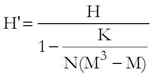
where K is sum of k3-k and k is the number of tied cases for a particular rank. H’ has a chi-square distribution with M – 1 degrees of freedom.
Although the chi-square statistic is commonly used, here we also report an alternative definition of the Friedman statistic based on the F distribution, with M – 1 and (N – 1)(M – 1) degrees of freedom, which is said to produce more accurate results (see Conover, W. J. 1999, p. 301). This version of the Friedman statistic is computed as follows: First the ranks (Rij, i = 1, …, N, j = 1, …, M) in each row and then their column totals are found (Rj, j = 1, …, M). The test statistic is defined as:
![]()
where:
![]()
![]()
The test statistic displayed is corrected for ties. The output includes rank sum and mean rank for each variable and correction for ties. The one-tail probability is reported using both chi-square distribution with M – 1 degrees of freedom and F-distribution with N – 1 and (N – 1)(M – 1) degrees of freedom.
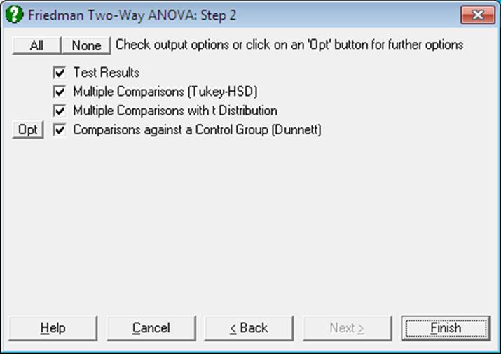
6.5.4.2. Friedman ANOVA Multiple Comparisons
If the null hypothesis is rejected as result of the Friedman’s test, then a multiple comparison can be run to find out which column effects are different.
Multiple comparisons with rank sums (Tukey-HSD)
Nonparametric Multiple Comparisons are performed in a way similar to the Tukey-HSD test using rank sums. The standard error is computed as:
![]()
Multiple comparisons with t-distribution
Comparisons are made using rank sums and the t-distribution. The standard error is computed as:
![]()
Comparisons against a control group (Dunnett)
If each group of data is to be tested against a control group then select this option. The standard error is computed as follows:
![]()
The only difference between the Dunnett test introduced here and the Dunnett test per se is that here the group rank sums are used while the latter uses group mean ranks.
6.5.4.3. Friedman ANOVA Examples
Example 1
Example 10.5 on p. 286 from Armitage & Berry (2002). Clotting times (min) of plasma from eight subjects, treated by four methods are given. The null hypothesis “there is no difference between the four treatments” is tested.
Open NONPARM1, select Statistics 1 → Nonparametric Tests (Multisample) → Friedman Two-Way ANOVA and select Treatment 1 to Treatment 4 (C23 to C26) as [Variable]s. Select Test Results as the only output option to obtain the following results:
Friedman Two-Way ANOVA
|
|
Cases |
Rank Sum |
Mean Rank |
|
Treatment 1 |
8 |
11.0000 |
1.3750 |
|
Treatment 2 |
8 |
16.0000 |
2.0000 |
|
Treatment 3 |
8 |
23.5000 |
2.9375 |
|
Treatment 4 |
8 |
29.5000 |
3.6875 |
|
Total |
32 |
80.0000 |
2.5000 |
|
Number of Columns = |
4 |
|
Number of Rows = |
8 |
|
Correction for Ties = |
0.0125 |
|
Chi-Square Statistic = |
15.1519 |
|
Degrees of Freedom = |
3 |
|
Right-Tail Probability = |
0.00169 |
|
F(3,21) = |
11.9871 |
|
Right-Tail Probability = |
0.0001 |
Both tests are significant at the 1% level. Hence reject the null hypothesis.
Example 2
Example 12.5 on p. 278 from Zar, J. H. (2010). A researcher wants to test the null hypothesis “time for effectiveness is the same for all three anesthetics”, or in other words that all means are the same against the alternative hypothesis that they are not all equal.
Open NONPARM1, select Statistics 1 → Nonparametric Tests (Multisample) → Friedman Two-Way ANOVA and include Treatment A to Treatment C (C40 to C42) in the analysis by clicking [Variable]. Check the Test Results output option only to obtain the following results:
Friedman Two-Way ANOVA
|
|
Cases |
Rank Sum |
Mean Rank |
|
Treatment A |
5 |
6.0000 |
1.2000 |
|
Treatment B |
5 |
15.0000 |
3.0000 |
|
Treatment C |
5 |
9.0000 |
1.8000 |
|
Total |
15 |
30.0000 |
2.0000 |
|
Number of Columns = |
3 |
|
Number of Rows = |
5 |
|
Correction for Ties = |
0.0000 |
|
Chi-Square Statistic = |
8.4000 |
|
Degrees of Freedom = |
2 |
|
Right-Tail Probability = |
0.0150 |
|
F(2,8) = |
21.0000 |
|
Right-Tail Probability = |
0.0007 |
As the right tail probability is less than 5% reject the null hypothesis.
Example 3
Example 1 on p. 371, Conover, W. J. (1999). A researcher wants to test the null hypothesis “the treatments in blocks (i.e. columns) have identical effects” at a 95% confidence level.
Open NONPARM1, select Statistics 1 → Nonparametric Tests (Multisample) → Friedman Two-Way ANOVA and include Grass 1 to Grass 4 (C31 to C34) in the analysis by clicking [Variable]. Select only the Test Results and Multiple comparisons with t-distribution output options to obtain the following results:
Friedman Two-Way ANOVA
|
|
Cases |
Rank Sum |
Mean Rank |
|
Grass 1 |
12 |
38.0000 |
3.1667 |
|
Grass 2 |
12 |
23.5000 |
1.9583 |
|
Grass 3 |
12 |
24.5000 |
2.0417 |
|
Grass 4 |
12 |
34.0000 |
2.8333 |
|
Total |
48 |
120.0000 |
2.5000 |
|
Number of Columns = |
4 |
|
Number of Rows = |
12 |
|
Correction for Ties = |
0.0583 |
|
Chi-Square Statistic = |
8.0973 |
|
Degrees of Freedom = |
3 |
|
Right-Tail Probability = |
0.0440 |
|
F(3,33) = |
3.1922 |
|
Right-Tail Probability = |
0.0362 |
Since the right tail probability is less than 5%, reject the null hypothesis. Therefore, we can proceed with Multiple Comparisons to find out which treatments are different.
Multiple Comparisons with t Distribution
Method: 95% t interval.
** denotes significantly different pairs. Vertical bars show homogeneous subsets.
A pairwise test result is significant if its q stat value is greater than the table q.
|
Group |
Cases |
Rank Sum |
Grass 2 |
Grass 3 |
Grass 4 |
Grass 1 |
|
|
Grass 2 |
12 |
23.5000 |
|
|
|
** |
| |
|
Grass 3 |
12 |
24.5000 |
|
|
|
** |
| |
|
Grass 4 |
12 |
34.0000 |
|
|
|
|
|| |
|
Grass 1 |
12 |
38.0000 |
** |
** |
|
|
| |
|
Comparison |
Difference |
Standard Error |
q Stat |
Table q |
Probability |
|
Grass 1 – Grass 2 |
14.5000 |
5.6434 |
2.5694 |
2.0345 |
0.0149 |
|
Grass 4 – Grass 2 |
10.5000 |
5.6434 |
1.8606 |
2.0345 |
0.0717 |
|
Grass 3 – Grass 2 |
1.0000 |
5.6434 |
0.1772 |
2.0345 |
0.8604 |
|
Grass 1 – Grass 3 |
13.5000 |
5.6434 |
2.3922 |
2.0345 |
0.0226 |
|
Grass 4 – Grass 3 |
9.5000 |
5.6434 |
1.6834 |
2.0345 |
0.1017 |
|
Grass 1 – Grass 4 |
4.0000 |
5.6434 |
0.7088 |
2.0345 |
0.4834 |
|
Comparison |
Lower 95% |
Upper 95% |
Result |
|
Grass 1 – Grass 2 |
3.0183 |
25.9817 |
** |
|
Grass 4 – Grass 2 |
-0.9817 |
21.9817 |
|
|
Grass 3 – Grass 2 |
-10.4817 |
12.4817 |
|
|
Grass 1 – Grass 3 |
2.0183 |
24.9817 |
** |
|
Grass 4 – Grass 3 |
-1.9817 |
20.9817 |
|
|
Grass 1 – Grass 4 |
-7.4817 |
15.4817 |
|
|
Homogeneous Subsets: |
|
|
Group 1: |
Grass 2 Grass 3 Grass 4 |
|
Group 2: |
Grass 4 Grass 1 |
The overall conclusion is that Grass 1/2 and Grass 1/3 are different.