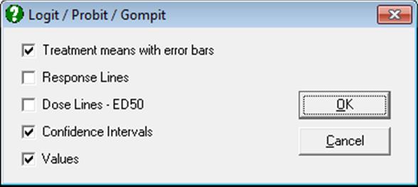
10.3. Quantal Response Method
Parallel line models can be fitted using one of logit, probit, gompit (clolglog) or loglog link functions. Asymmetric dose structures and multiple test preparations are supported. To test the validity of assay a Weighted ANOVA table (including non-parallelism and non-linearity tests) is displayed. Output includes estimates of effective dose (or lethal dose) for any user-defined percentile (including ED50, EC50 or LD50), the potency ratio and their confidence limits.
10.3.1. Quantal Response Variable Selection
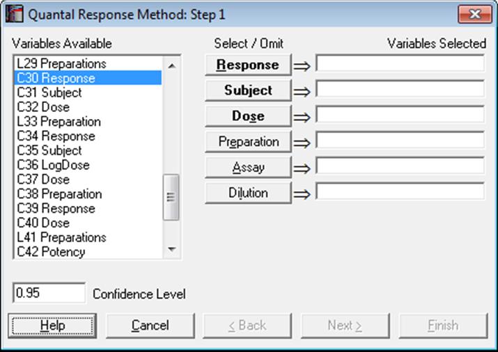
The first variable [Response] represents the number subjects responding positively (or negatively) to the test and the second [Subject] contains the total number of subjects in that group. Therefore, the following relation should hold for each case:
0 ≤ Response ≤ Subject
If some cases do not conform to this, then the analysis will be aborted. Cases with a zero Subject will be considered missing.
As in other bioassay procedures, a [Dose] variable should also be selected. However, the choice of a [Preparation] variable is optional. If a [Preparation] variable is not selected, then an ED50 estimate can still be computed, fitting a single line (instead of parallel lines) on all data points.
Designs can be unbalanced, i.e. the number of replicates for each dose-preparation combination may be different, dose levels for standard and test preparations may be different, there can be more than one test preparation, but the first five characters of the standard preparation label should be “stand” or “refer” in any language (capitalisation is not significant). Otherwise the first preparation encountered in the [Preparation] column will be considered as the standard. For the two optional variables [Assay] and [Dilution], see sections 10.0.4. Multiple Assays with Combination and 10.0.2. Doses, Dilutions and Potency respectively.
The next dialogue asks for the following convergence and model parameters.
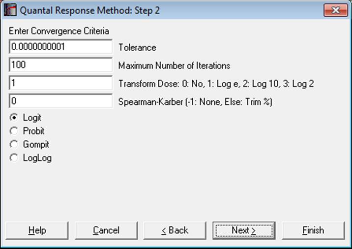
Tolerance: This value is used to control the sensitivity of the maximum likelihood procedure employed. Under normal circumstances, you do not need to change this value. If convergence cannot be achieved, then larger values of this parameter can be tried by removing one or more zeros.
Maximum Number of Iterations: When convergence cannot be achieved with the default value of 100 function evaluations, a higher value can be tried.
Dose Transformation: It is possible to transform the dose variable by natural (default), 10 or 2-based logarithm or leave it untransformed.
Spearman-Karber: When a non-negative percentage is entered, ED50 and its confidence limits are also computed using the Spearman-Karber method. When this box contains a negative value, Spearman-Karber results are not reported.
Link Function: Select the model to be estimated; logit, probit, gompit (cloglog) or loglog.
Predictions (Interpolations): Predictions can be obtained for response or dose values using the estimated model parameters. For details see section 10.0.7. Prediction, Interpolation, Extrapolation.
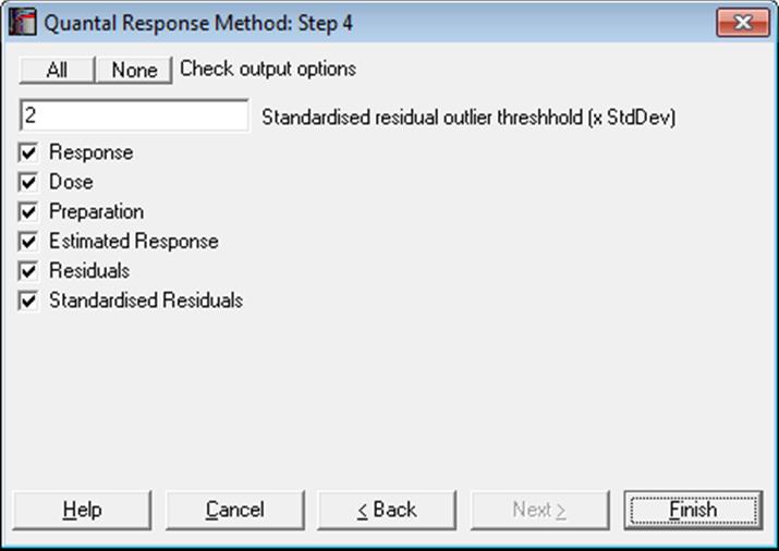
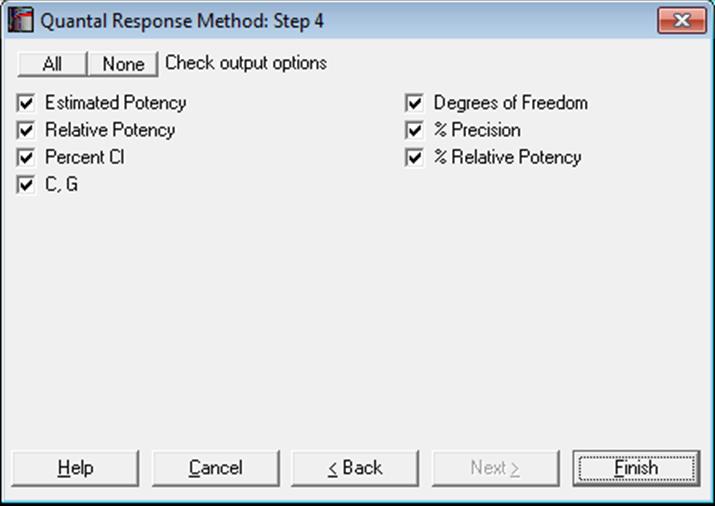
10.3.2. Quantal Response Output Options
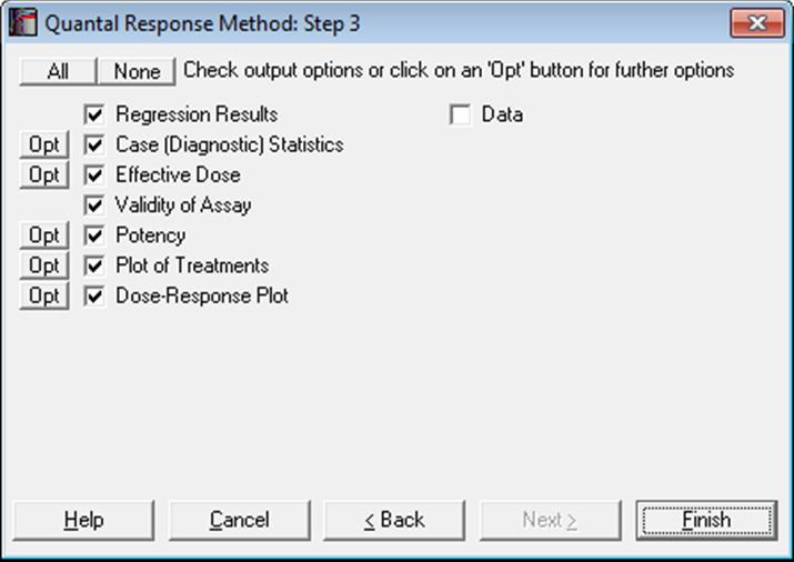
10.3.2.1. Regression Results
The maximum likelihood model is constructed as a regression without a constant term (i.e. through the origin), with independent variables consisting of the transformed dose variable and a set of m dummy variables created from the preparations variable. When the convergence is achieved, the coefficient for the dose variable represents the estimated common slope and coefficients for the dummy variables represent the estimated intercept for each preparation.
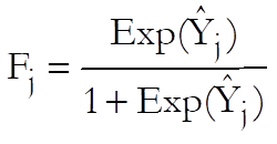
The dependent variable is obtained from the response and
subject variables. Let ![]() be
the expected value for case j. Then:
be
the expected value for case j. Then:
Logit:
Probit:
![]()
Gompit (cloglog):
![]()
Loglog:
![]()
For further details see 7.2.5.1. Logit / Probit / Gompit Model Description.
A Newton-Raphson type maximum likelihood algorithm is employed to minimise the negative of the log likelihood function. The nature of this method implies that a solution (convergence) cannot always be achieved. In such cases, you are advised to edit the convergence parameters provided, in order to find the right levels for the particular problem at hand.
10.3.2.2. Case (Diagnostic) Statistics
10.3.2.3. Effective Dose (or Lethal Dose)
By default, ED50 (or EC50 or LD50) values and their fiducial confidence limits are computed for all preparations. If a non-negative percentage is entered in the Spearman-Karber box, ED50 values, their confidence limits and actual percentage trim used are also displayed for each preparation using this method. If the [Preparation] variable is not selected or contains only one value, then an ED50 estimate will still be calculated, fitting a single line (instead of parallel lines) on all data points. Let d be the user-supplied effective dose (or lethal dose) quantile. Then for the logit model compute:
![]()
and for the probit model:
Y = Critical value of (1 – d) from inverse standard normal distribution.
The effective dose for preparation i is then found as:
![]()
where ![]() is
the intercept for preparation i and
is
the intercept for preparation i and ![]() is the common slope.
is the common slope.
To calculate the confidence limits of Mi first define:
![]()
where Vb is the variance of common slope and ![]() is the critical value from normal
distribution.
is the critical value from normal
distribution.
The confidence interval for potency ratio of each test preparation is defined as:
![]()
where:
![]()
and Vss, Vii and Vsi are the elements of covariance matrix of regression coefficients for standard and preparation i.
The trimmed Spearman-Karber (or Kaerber) and its confidence interval are computed as described in Hamilton at al (1977). If the consecutive response values are not monotonically increasing (or decreasing) their average is used. If the trim entered by the user has no solution, then the minimum trim estimated by the program is used. For each preparation, the percentage trim entered and the trim used by the program are displayed.
Effective Dose
|
|
Effective Dose |
Lower 95% |
Upper 95% |
Trim Entered |
Trim Used |
|
Standard S ED50 |
2.3489 |
1.9291 |
2.8956 |
|
|
|
Spearman-Karber |
2.3391 |
1.8891 |
2.8961 |
0.00% |
9.09% |
|
Preparation T ED50 |
2.0477 |
1.6716 |
2.5166 |
|
|
|
Spearman-Karber |
1.9703 |
1.5878 |
2.4450 |
0.00% |
9.09% |
If you wish to compute other effective dose values then, on the Output Options Dialogue, click the [Opt] button situated to the left of the Effective Dose option. A further dialogue pops up asking for entry of a value between 0 and 1.
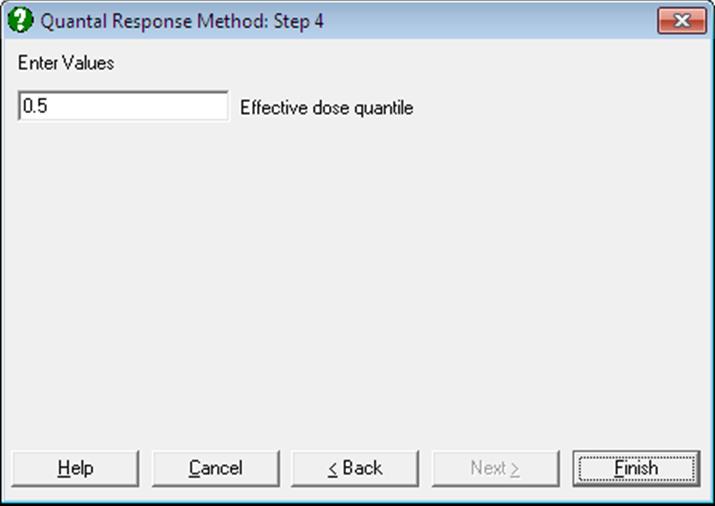
The program will then output the effective dose and its confidence limits for this value, as well as its complementary value, for all preparations. For instance, if 0.9 is entered, ED10 and ED90 values will be computed and the output will look like as follows:
|
|
Effective Dose |
Lower 95% |
Upper 95% |
|
Standard ED10 |
4.4731 |
3.5712 |
5.2983 |
|
ED90 |
28.2233 |
23.6956 |
35.6538 |
|
Unknown ED10 |
6.6911 |
5.2925 |
8.0338 |
|
ED90 |
42.2176 |
34.4987 |
55.0306 |
10.3.2.4. Validity of Assay
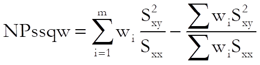
Unlike Parallel Line Method and Slope Ratio Method, in Quantal Response Method the validity of assay is based on weighted sums of squares. This allows us to perform chi-square tests for various model parameters.
Non-linearity test:
![]()
where Sxx, Syy and Sxy are sum of squares as defined in Finney, D. J. (1978) p. 372. The test statistic has (n – 4) degrees of freedom.
Non-parallelism test:
The test statistic has (m – 1) degrees of freedom.
Weighted ANOVA
|
|
Sum of Squares |
Chi-Square |
DoF |
Probability |
Pass/Fail |
|
Preparations |
0.066 |
0.066 |
1 |
0.7969 |
Pass |
|
Regression |
33.975 |
33.975 |
1 |
0.0000 |
Pass |
|
Non-parallelism |
0.001 |
0.001 |
1 |
0.9743 |
Pass |
|
Non-linearity |
1.921 |
1.921 |
4 |
0.7502 |
Pass |
|
Standard S Non-linearity |
0.851 |
0.851 |
2 |
0.6533 |
Pass |
|
Preparation T Non-linearity |
1.070 |
1.070 |
2 |
0.5856 |
Pass |
|
Treatments |
35.964 |
35.964 |
7 |
0.0000 |
Pass |
|
Residual |
|
|
|
|
|
|
Total |
35.964 |
|
7 |
|
|
|
R-squared |
0.947 |
|
|
|
**Fail** |
10.3.2.5. Potency
The relative potency for test preparation i is found as:
![]()
where ![]() and
and
![]() are the intercepts
for test i and standard preparations and
are the intercepts
for test i and standard preparations and ![]() is the common slope.
is the common slope.
To calculate the confidence limits of Mi first define:
![]()
where Vb is the variance of common slope and ![]() is the critical value from normal
distribution.
is the critical value from normal
distribution.
First define:
![]()
![]()
The fiducial confidence interval for potency ratio of each test preparation is defined as:
![]()
where:
![]()
Mi is the relative potency and MiL and MiU are the confidence limits for the relative potency. The estimated potency and its confidence interval are obtained by multiplying these relative values by the assumed potency supplied by the user for each test preparation separately.
The approximate variance of Mi is:
![]()
Weights are computed after the estimated potency and its confidence interval are found:
![]()
and % Precision is:
![]()
If the data column [Dose] contains the actual dose levels administered in original dose units, we will obtain the estimated potency and its confidence limits in the same units. If, however, the [Dose] column contains unitless relative dose levels, then we may need to perform further calculations to obtain the estimated potency in original units. To do that you can enter assigned potency of the standard, assumed potency of each test preparation and pre-dilutions for all preparations including the standard in a data column and select it as [Dilution] variable. UNISTAT will then calculate the estimated potency as described in section 10.0.2. Doses, Dilutions and Potency. Also see section 10.0.3. Potency Calculation Example.
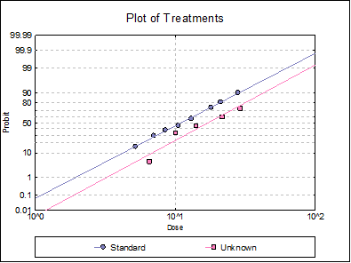
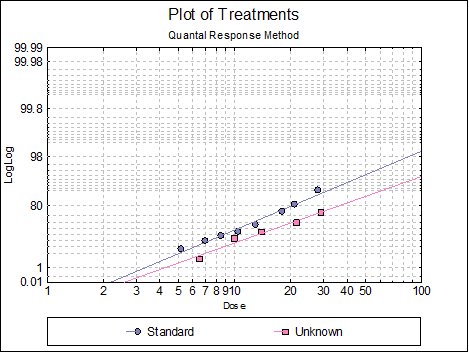
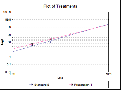
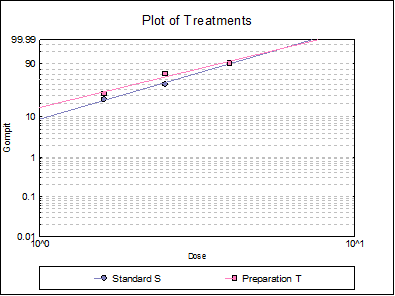
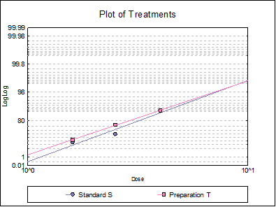
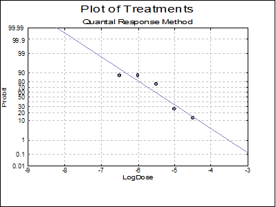
10.3.2.6. Plot of Treatments
Response ratios are plotted on a logit, probit, gompit or loglog Y-axis (see Scale Type), versus log of dose, according to the model selected. A line of best fit is also drawn for each preparation. If you want to edit the properties of the graph, you can send it to Graphics Editor by clicking on the [Opt] button situated to the left of the plot option. The Edit → Data Series dialogue on the graphics window menu provides you with necessary controls to edit all aspects of the plot.
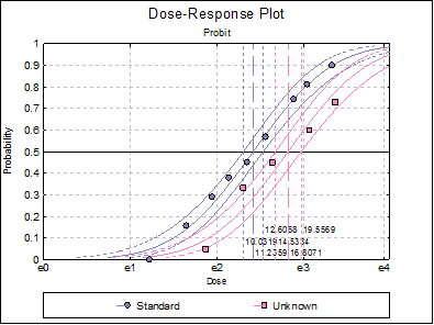
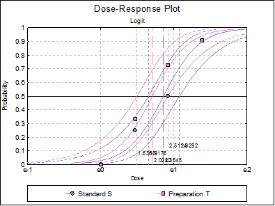
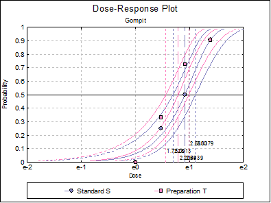
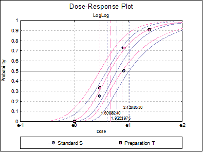
10.3.2.7. Dose-Response Plot
A dose-response curve will be drawn for each preparation. For each curve it is possible to display fiducial limits, ED50, and the fiducial limits for ED50.
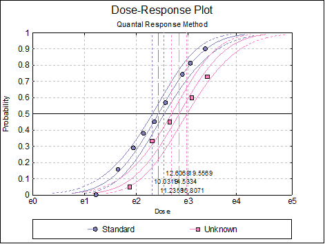
Selecting Edit → Dose-Response Plot… (or double-clicking on the graph area) will pop a dialogue where what is displayed on the plot can be controlled.
10.3.3. Quantal Response Examples
Example 1
Data is given in p. 4371 of European Pharmacopoeia (9th Edition) Table 5.3.1.-I.
Open BIOPHARMA9 and select Bioassay → Quantal Response Method. From the Variable Selection Dialogue select columns C35, C36, C37, L38 and L39 respectively as [Response], [Subject], [Dose], [Preparation] and [Dilution]. Click [Next], select Probit model and leave other entries unchanged.
Quantal Response Method
Valid Number of Cases: 8, 0 Omitted
Model selected: Logit
Regression Results
|
|
Coefficient |
Standard Error |
Z-Statistic |
2-Tail Probability |
Lower 90% |
Upper 90% |
|
Common Slope |
2.4011 |
0.4170 |
5.7582 |
0.0000 |
1.7152 |
3.0869 |
|
Intercept Standard S |
-2.0504 |
0.4086 |
-5.0176 |
0.0000 |
-2.7226 |
-1.3783 |
|
Intercept Preparation T |
-1.7208 |
0.3829 |
-4.4945 |
0.0000 |
-2.3506 |
-1.0911 |
|
Residual Variance = |
0.4781 |
|
Degrees of Freedom = |
5 |
Case (Diagnostic) Statistics
|
|
Response |
Subject |
Dose |
Preparation |
|
1 |
0 |
12 |
1 |
Standard S |
|
2 |
3 |
12 |
1.6 |
Standard S |
|
3 |
6 |
12 |
2.5 |
Standard S |
|
4 |
10 |
11 |
4 |
Standard S |
|
5 |
0 |
11 |
1 |
Preparation T |
|
** 6 |
4 |
12 |
1.6 |
Preparation T |
|
** 7 |
8 |
11 |
2.5 |
Preparation T |
|
8 |
10 |
11 |
4 |
Preparation T |
|
|
Estimated Response |
Residuals |
Standardised Residuals |
Probability |
|
1 |
0.2419 |
-0.2419 |
-0.3499 |
0.0202 |
|
2 |
2.1395 |
0.8605 |
1.2445 |
0.1783 |
|
3 |
6.7138 |
-0.7138 |
-1.0323 |
0.5595 |
|
4 |
9.8935 |
0.1065 |
0.1541 |
0.8994 |
|
5 |
0.2218 |
-0.2218 |
-0.3207 |
0.0202 |
|
** 6 |
2.1395 |
1.8605 |
2.6907 |
0.1783 |
|
** 7 |
6.1543 |
1.8457 |
2.6692 |
0.5595 |
|
8 |
9.8935 |
0.1065 |
0.1541 |
0.8994 |
Cases marked by ‘**’ are outliers at 2 x Standard Deviation.
Effective Dose
|
|
Effective Dose |
Lower 95% |
Upper 95% |
Trim Entered |
Trim Used |
|
Standard S ED50 |
2.3489 |
1.9291 |
2.8956 |
|
|
|
Spearman-Karber |
2.3391 |
1.8891 |
2.8961 |
0.00% |
9.09% |
|
Preparation T ED50 |
2.0477 |
1.6716 |
2.5166 |
|
|
|
Spearman-Karber |
1.9703 |
1.5878 |
2.4450 |
0.00% |
9.09% |
Weighted ANOVA
|
|
Sum of Squares |
Chi-Square |
DoF |
Probability |
Pass/Fail |
|
Preparations |
0.066 |
0.066 |
1 |
0.7969 |
Pass |
|
Regression |
33.975 |
33.975 |
1 |
0.0000 |
Pass |
|
Non-parallelism |
0.001 |
0.001 |
1 |
0.9743 |
Pass |
|
Non-linearity |
1.921 |
1.921 |
4 |
0.7502 |
Pass |
|
Standard S Non-linearity |
0.851 |
0.851 |
2 |
0.6533 |
Pass |
|
Preparation T Non-linearity |
1.070 |
1.070 |
2 |
0.5856 |
Pass |
|
Treatments |
35.964 |
35.964 |
7 |
0.0000 |
Pass |
|
Residual |
|
|
|
|
|
|
Total |
35.964 |
|
7 |
|
|
|
R-squared |
0.947 |
|
|
|
**Fail** |
Potency
Assigned potency of Standard S: 132 IU/vial
Assumed potency of Preparation T: 140 IU/vial
|
|
Estimated Potency |
Lower 95% |
Upper 95% |
|
Preparation T |
160.5974 |
120.9660 |
215.1559 |
|
|
Relative Potency |
Lower 95% |
Upper 95% |
|
Preparation T |
114.71% |
86.40% |
153.68% |
|
|
Percent CI |
Lower 95% |
Upper 95% |
|
Preparation T |
100.00% |
75.32% |
133.97% |
|
G = |
0.1131 |
|
C = |
1.1275 |
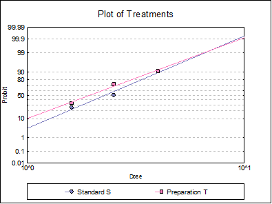
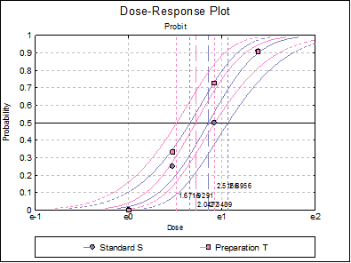
Table 5.3.2.-I. also gives the results for logit and gompit methods. Click on the [Last Dialogue] button on the Output Medium Toolbar. This will display the Output Options Dialogue again. Click [Back], select the Logit model, click [Next] and select only the Potency output option.
Quantal Response Method
Valid Number of Cases: 8, 0 Omitted
Model selected: Logit
Potency
Assigned potency of Standard S: 132 IU/vial
Assumed potency of Preparation T: 140 IU/vial
|
|
Estimated Potency |
Lower 95% |
Upper 95% |
|
Preparation T |
162.8590 |
121.1311 |
221.1056 |
|
|
Relative Potency |
Lower 95% |
Upper 95% |
|
Preparation T |
116.33% |
86.52% |
157.93% |
|
|
Percent CI |
Lower 95% |
Upper 95% |
|
Preparation T |
100.00% |
74.38% |
135.77% |
Select the Gompit model and repeat the analysis.
Quantal Response Method
Valid Number of Cases: 8, 0 Omitted
Model selected: Logit
Potency
Assigned potency of Standard S: 132 IU/vial
Assumed potency of Preparation T: 140 IU/vial
|
|
Estimated Potency |
Lower 95% |
Upper 95% |
|
Preparation T |
158.3126 |
118.7082 |
213.2961 |
|
|
Relative Potency |
Lower 95% |
Upper 95% |
|
Preparation T |
113.08% |
84.79% |
152.35% |
|
|
Percent CI |
Lower 95% |
Upper 95% |
|
Preparation T |
100.00% |
74.98% |
134.73% |
Select the LogLog model and repeat the analysis.
Quantal Response Method
Valid Number of Cases: 8, 0 Omitted
Model selected: Logit
Potency
Assigned potency of Standard S: 132 IU/vial
Assumed potency of Preparation T: 140 IU/vial
|
|
Estimated Potency |
Lower 95% |
Upper 95% |
|
Preparation T |
159.1364 |
120.0325 |
211.3075 |
|
|
Relative Potency |
Lower 95% |
Upper 95% |
|
Preparation T |
113.67% |
85.74% |
150.93% |
|
|
Percent CI |
Lower 95% |
Upper 95% |
|
Preparation T |
100.00% |
75.43% |
132.78% |
Example 2
Data is given in p. 4373 of European Pharmacopoeia (9th Edition) Table 5.3.3.-I.
Open BIOPHARMA9 and select Bioassay → Quantal Response Method. From the Variable Selection Dialogue select columns C40 to C42, Response, Subject, LogDose respectively as [Response], [Subject], [Dose]. You do not need to select a [Preparation] variable, though you can also select C43 Preparation as [Preparation] as it contains only one value. Click [Next], select Probit model and select the dose transformation None, since the data is already logged base 10. On the Output Options Dialogue click [Finish]. The following output is obtained:
Quantal Response Method
Valid Number of Cases: 10, 0 Omitted
Model selected: Probit
Regression Results
|
|
Coefficient |
Standard Error |
Z-Statistic |
2-Tail Probability |
Lower 95% |
Upper 95% |
|
Common Slope |
-1.4880 |
0.3063 |
-4.8580 |
0.0000 |
-2.0883 |
-0.8877 |
|
Intercept 1 |
-7.9314 |
1.6586 |
-4.7820 |
0.0000 |
-11.1822 |
-4.6806 |
Effective Dose
|
|
Effective Dose |
Lower 95% |
Upper 95% |
|
1 ED50 |
-5.3302 |
-5.6568 |
-5.0022 |
Weighted ANOVA
|
|
Sum of Squares |
Chi-Square |
DoF |
Probability |
Pass/Fail |
|
Preparations |
0.000 |
0.000 |
0 |
* |
* |
|
Regression |
23.337 |
23.337 |
1 |
0.0000 |
Pass |
|
Non-parallelism |
0.000 |
0.000 |
0 |
* |
* |
|
Non-linearity |
2.711 |
2.711 |
8 |
0.9512 |
Pass |
|
Treatments |
26.049 |
26.049 |
9 |
0.0020 |
Pass |
|
Residual |
|
|
|
|
|
|
Total |
26.049 |
|
9 |
|
|
|
R-squared |
0.896 |
|
|
|
|
Remember that the dose data were already logged base 10. Applying the back-transformation (again base 10):
-MT + Log(1000/50)
and reversing the limits we obtain:
|
|
Effective Dose |
Lower 95% |
Upper 95% |
|
1 ED50 |
6.6313 |
6.3033 |
6.9578 |
Example 3
Table 18.2.1. on p. 376 from Finney, D. J. (1978) gives data for an unbalanced assay with one test preparation. Finney gives the results in Table 18.3.1. on p. 380.
Open BIOFINNEY and select Bioassay → Quantal Response Method. From the Variable Selection Dialogue select columns C20 to C23 respectively as [Response], [Subject], [Dose] and [Preparation].
Standard and test preparations are equipotent. The standard has an assigned potency of 20 IU/vial and the test preparation has an assumed potency of 20 IU/vial. Create a new column of data as follows and select it as [Dilution] variable.
20 IU/vial
1
20 IU/vial
1
For further information see section 10.0.2. Doses, Dilutions and Potency.
Click [Next], select Probit model and leave other entries unchanged.
Quantal Response Method
Valid Number of Cases: 14, 0 Omitted
Model selected: Probit
Regression Results
|
|
Coefficient |
Standard Error |
Z-Statistic |
2-Tail Probability |
Lower 90% |
Upper 90% |
|
Common Slope |
1.3914 |
0.1234 |
11.2782 |
0.0000 |
1.1885 |
1.5944 |
|
Intercept Standard |
-3.3660 |
0.3061 |
-10.9960 |
0.0000 |
-3.8695 |
-2.8625 |
|
Intercept Unknown |
-3.9263 |
0.3520 |
-11.1554 |
0.0000 |
-4.5053 |
-3.3474 |
|
Residual Variance = |
2.3831 |
|
Degrees of Freedom = |
11 |
Case (Diagnostic) Statistics
|
|
Response |
Subject |
Dose |
Preparation |
|
1 |
0 |
33 |
3.4 |
Standard |
|
2 |
5 |
32 |
5.2 |
Standard |
|
3 |
11 |
38 |
7 |
Standard |
|
4 |
14 |
37 |
8.5 |
Standard |
|
5 |
18 |
40 |
10.5 |
Standard |
|
6 |
21 |
37 |
13 |
Standard |
|
7 |
23 |
31 |
18 |
Standard |
|
8 |
30 |
37 |
21 |
Standard |
|
9 |
27 |
30 |
28 |
Standard |
|
** 10 |
2 |
40 |
6.5 |
Unknown |
|
11 |
10 |
30 |
10 |
Unknown |
|
** 12 |
18 |
40 |
14 |
Unknown |
|
** 13 |
21 |
35 |
21.5 |
Unknown |
|
** 14 |
27 |
37 |
29 |
Unknown |
|
|
Estimated Response |
Residuals |
Standardised Residuals |
Probability |
|
1 |
1.5884 |
-1.5884 |
-1.0289 |
0.0481 |
|
2 |
4.5393 |
0.4607 |
0.2984 |
0.1419 |
|
3 |
9.6950 |
1.3050 |
0.8453 |
0.2551 |
|
4 |
12.9095 |
1.0905 |
0.7064 |
0.3489 |
|
5 |
18.4982 |
-0.4982 |
-0.3227 |
0.4625 |
|
6 |
21.4748 |
-0.4748 |
-0.3076 |
0.5804 |
|
7 |
23.0640 |
-0.0640 |
-0.0414 |
0.7440 |
|
8 |
29.8926 |
0.1074 |
0.0696 |
0.8079 |
|
9 |
26.9414 |
0.0586 |
0.0380 |
0.8980 |
|
** 10 |
8.9266 |
-6.9266 |
-4.4869 |
0.2232 |
|
11 |
13.0679 |
-3.0679 |
-1.9873 |
0.4356 |
|
** 12 |
24.8085 |
-6.8085 |
-4.4104 |
0.6202 |
|
** 13 |
28.5854 |
-7.5854 |
-4.9136 |
0.8167 |
|
** 14 |
33.5394 |
-6.5394 |
-4.2361 |
0.9065 |
Cases marked by ‘**’ are outliers at 2 x Standard Deviation.
Effective Dose
|
|
Effective Dose |
Lower 95% |
Upper 95% |
Trim Entered |
Trim Used |
|
Standard ED50 |
11.2359 |
10.0319 |
12.6068 |
|
|
|
Spearman-Karber |
11.0745 |
9.8289 |
12.4780 |
0.00% |
10.00% |
|
Unknown ED50 |
16.8071 |
14.5334 |
19.5569 |
|
|
|
Spearman-Karber |
16.0704 |
12.9779 |
19.8997 |
0.00% |
27.03% |
Weighted ANOVA
|
|
Sum of Squares |
Chi-Square |
DoF |
Probability |
Pass/Fail |
|
Preparations |
0.594 |
0.594 |
1 |
0.4407 |
Pass |
|
Regression |
130.268 |
130.268 |
1 |
0.0000 |
Pass |
|
Non-parallelism |
0.282 |
0.282 |
1 |
0.5951 |
Pass |
|
Non-linearity |
5.421 |
5.421 |
10 |
0.8614 |
Pass |
|
Standard Non-linearity |
2.058 |
2.058 |
7 |
0.9565 |
Pass |
|
Unknown Non-linearity |
3.363 |
3.363 |
3 |
0.3390 |
Pass |
|
Treatments |
136.566 |
136.566 |
13 |
0.0000 |
Pass |
|
Residual |
|
|
|
|
|
|
Total |
136.566 |
|
13 |
|
|
|
R-squared |
0.958 |
|
|
|
Pass |
Potency
Assigned potency of Standard: 20 IU/vial
Assumed potency of Unknown: 20 IU/vial
|
|
Estimated Potency |
Lower 95% |
Upper 95% |
|
Unknown |
13.3704 |
11.0678 |
16.0812 |
|
|
Relative Potency |
Lower 95% |
Upper 95% |
|
Unknown |
66.85% |
55.34% |
80.41% |
|
|
Percent CI |
Lower 95% |
Upper 95% |
|
Unknown |
100.00% |
82.78% |
120.28% |