9.3.1. Variable Control Charts
These methods (which are also known as Shewhart charts) attempt to control quality characteristics that can be expressed as numerical measures. Examples include the diameter of a piston, the weight of beverage placed in a bottle, etc. The general approach is straightforward: simply extract samples of a certain size from the process, produce charts for the variability of those samples and their closeness to target specifications. In an application, it is general practice to ensure that the variability is in control before examining the central tendency. The variability is controlled with the R Chart, S Chart and Variance Chart in UNISTAT. The central tendency is controlled with the X Bar Chart, Moving Average Charts and CUSUM Chart.
9.3.1.0. Overview
Two types of data can be analysed.
9.3.1.0.1. Raw Values and Samples

When this method is used, you will need to select one column that contains the data values by clicking on [Variable] and a second column that specifies which sample the value is associated with by clicking on [Sample]. The sample column is like a factor column, in that the levels within the column are used to classify the data into groups, but there is also an order implied in these classes. It is assumed that sample numbers with higher values are taken later in time, but the sample numbers need not be strictly sequential. It is also possible to use a date column as the sample column. In this case each measurement taken on the same day will be in the same sample.
It must be noted here that all Variable Control Charts involve grouping of the original raw data and the points on the plot will correspond to samples rather than the individual observations. For instance, if you have a [Variable] column with 200 observations and a [Sample] column which also has 200 rows but only 5 distinct values, then Variable Control Charts will produce a graph with 5 points only, corresponding to each sample. One exception to this is X Chart (Levey-Jennings), which does not involve a grouping of observations. It will plot all 200 observations and the [Sample] column will not play a role in the appearance of the curve. However, we assume that there is an underlying sample here, in parallel with other Variable Control Charts. In X Chart, the [Sample] column can be used for labelling purposes, particularly in marking which outlying points belong to which sample.
9.3.1.0.2. Summary Data
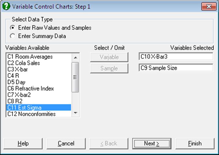
When this data option is selected, each row in the data matrix is assumed to represent a sample. You may select up to four columns containing sample sizes, means, standard errors and the sample ranges by clicking on [Size], [Mean], [Std Dev] and [Range] respectively.
Only one of standard error and range columns must be selected. If all the variables are not selected from the Variables Available list, output options will be reduced in the following way:
Sample size not specified: UNISTAT will prompt for a common sample size to apply to all samples.
Mean not specified: The X Bar Chart, Moving Average Charts and CUSUM Chart will not be available.
Standard error not specified: The S Chart and Variance Chart will not be available.
Range not specified: The R Chart will not be available.
If the columns have been selected but within these columns values are missing, UNISTAT behaves in the following way. If the sample size is missing then the average sample size is used. If the mean value is missing then this row will be missing on X Bar Chart, Moving Average Charts and CUSUM Chart. If the standard error is missing then the row will be missing on S Chart and Variance Chart. If the range is missing then the row will be missing on an R Chart. If both standard error and range are missing then the row is considered to be missing.
9.3.1.0.3. Standard Error Estimation
In X Bar Chart, Moving Average Charts and CUSUM Chart the standard error for each sample is required. If the standard error for a sample is not given then it is estimated from the range within the given sample.
9.3.1.1. R Chart
In R Chart, the sample ranges are plotted in order to control the variability of a variable. The sample sizes should be small and fairly consistent. This chart only uses the two most extreme values from a sample and so is weaker than the S Chart. Also the true target level varies with the sample size. The R Chart does not account for this, and use the average sample size to estimate the target level. So samples should have sizes near this value.
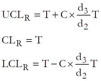
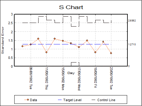
where:
· T is the target level. UNISTAT gives the mean range of the samples as the default value.
· C is the control line parameter.
· d2, d3 are known parameters dependent on sample size such that:
![]()
Example
Table 7.1 on p. 189 from Banks, Jerry (1989). X-bar and R values for Socket Dimensions are given in centimetres.
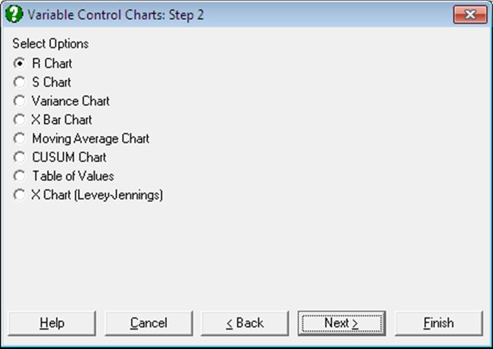
Open TIMESER and select Statistics 2 → Quality Control → Variable Control Charts. Select the data option 2 Enter Summary Data and X-Bar (C3) as [Mean] and R (C4) as [Range]. From the next dialogue select the sample size as 5 and from the next one R Chart as the output option. At the next dialogue leave the default values as follows:
· 2.7136E-02 Target Level
· 3 Control Line (* Sigma)
· 0 Warning Line (* Sigma)
· 0 MA Parameter (>1 MA, 1< EWMA)
· 0 Use Average N (0 No, Else Yes)
And finally, from the Output Options Dialogue click [Finish].
Variable Control Charts
R Chart
Size = 5.0000
Mean: X-bar
Range: R
‘*’ denotes sample outside control limits
|
Sample |
Value |
LCL |
UCL |
|
1 |
0.0350 |
0.0000 |
0.0574 |
|
2 |
0.0210 |
0.0000 |
0.0574 |
|
3 |
0.0380 |
0.0000 |
0.0574 |
|
4 |
0.0160 |
0.0000 |
0.0574 |
|
5 |
0.0280 |
0.0000 |
0.0574 |
|
6 |
0.0190 |
0.0000 |
0.0574 |
|
7 |
0.0390 |
0.0000 |
0.0574 |
|
8 |
0.0250 |
0.0000 |
0.0574 |
|
9 |
0.0160 |
0.0000 |
0.0574 |
|
10 |
0.0190 |
0.0000 |
0.0574 |
|
11 |
0.0370 |
0.0000 |
0.0574 |
|
12 |
0.0280 |
0.0000 |
0.0574 |
|
13 |
0.0320 |
0.0000 |
0.0574 |
|
14 |
0.0370 |
0.0000 |
0.0574 |
|
15 |
0.0240 |
0.0000 |
0.0574 |
|
16 |
0.0180 |
0.0000 |
0.0574 |
|
17 |
0.0330 |
0.0000 |
0.0574 |
|
18 |
0.0390 |
0.0000 |
0.0574 |
|
19 |
0.0190 |
0.0000 |
0.0574 |
|
20 |
0.0230 |
0.0000 |
0.0574 |
|
21 |
0.0270 |
0.0000 |
0.0574 |
|
22 |
0.0240 |
0.0000 |
0.0574 |
|
Target Level = |
0.0271 |
|
Average Sample Size = |
5.0000 |
|
Control Limits = |
3.0000 x Sigma |
|
Sigma = |
0.0117 |
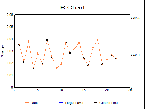
This shows that the range (and hence the variability) is under control and we can proceed to examine the central tendency.
9.3.1.2. S Chart
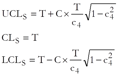
In S Chart the sample standard errors are plotted in order to control the variability of a variable. For large sample sizes this chart is more powerful than the R Chart.
where:
· T is the target level. UNISTAT gives the average standard deviation of the samples as the default value,
· C is the control line parameter.
· c4 is a known parameter dependent on sample size, n.
![]()
Example
Table 7.5 on p. 214 from Banks, Jerry (1989). Refractive Index of Fiber Optic Cable is given.
Open TIMESER and select Statistics 2 → Quality Control → Variable Control Charts. Select the data option 1 Enter Raw Values and Samples and Day (C5) as [Sample] and Refractive Index (C6) as [Variable]. From the next dialogue select S Chart and leave the default values as follows:
· 1.2715 Target Level
· 3 Control Line (* Sigma)
· 0 Warning Line (* Sigma)
· 0 MA Parameter (>1 MA, 1< EWMA)
· 0 Use Average N (0 No, Else Yes)
From the final output dialogue click [Finish] to obtain the following graph, which shows that the variability is under control.
Variable Control Charts
S Chart
Sample: Day
Variable: Refractive Index
‘*’ denotes sample outside control limits
|
Sample |
Value |
LCL |
UCL |
|
08/06/1992 Mon |
1.1466 |
0.0386 |
2.5044 |
|
09/06/1992 Tue |
1.2501 |
0.0386 |
2.5044 |
|
10/06/1992 Wed |
1.5948 |
0.0000 |
2.8813 |
|
11/06/1992 Thu |
0.8204 |
0.0000 |
2.6562 |
|
12/06/1992 Fri |
1.5870 |
0.0386 |
2.5044 |
|
15/06/1992 Mon |
1.4617 |
0.0000 |
2.8813 |
|
16/06/1992 Tue |
1.3307 |
0.2353 |
2.3077 |
|
17/06/1992 Wed |
1.0996 |
0.0000 |
2.8813 |
|
18/06/1992 Thu |
1.4828 |
0.0386 |
2.5044 |
|
19/06/1992 Fri |
0.8019 |
0.0000 |
2.6562 |
|
22/06/1992 Mon |
1.4166 |
0.0386 |
2.5044 |
|
23/06/1992 Tue |
0.7668 |
0.0000 |
2.6562 |
|
Target Level = |
1.2715 |
|
Average Sample Size = |
5.4167 |
|
Control Limits = |
3.0000 x Sigma |
|
Sigma = |
1.2715 |
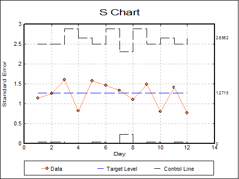
It is possible to edit the graph settings to display dates on the x-axis, instead row numbers.
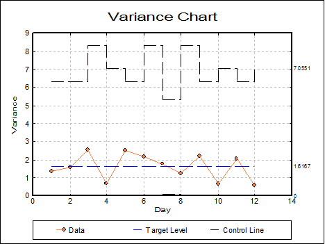
9.3.1.3. Variance Chart
This is simply the S Chart with all the values squared. Keeping the selections for the previous example we obtain:
Variable Control Charts
Variance Chart
Sample: Day
Variable: Refractive Index
‘*’ denotes sample outside control limits
|
Sample |
Value |
LCL |
UCL |
|
08/06/1992 Mon |
1.3147 |
0.0015 |
6.2719 |
|
09/06/1992 Tue |
1.5627 |
0.0015 |
6.2719 |
|
10/06/1992 Wed |
2.5433 |
0.0000 |
8.3017 |
|
11/06/1992 Thu |
0.6730 |
0.0000 |
7.0551 |
|
12/06/1992 Fri |
2.5187 |
0.0015 |
6.2719 |
|
15/06/1992 Mon |
2.1367 |
0.0000 |
8.3017 |
|
16/06/1992 Tue |
1.7707 |
0.0554 |
5.3253 |
|
17/06/1992 Wed |
1.2092 |
0.0000 |
8.3017 |
|
18/06/1992 Thu |
2.1987 |
0.0015 |
6.2719 |
|
19/06/1992 Fri |
0.6430 |
0.0000 |
7.0551 |
|
22/06/1992 Mon |
2.0067 |
0.0015 |
6.2719 |
|
23/06/1992 Tue |
0.5880 |
0.0000 |
7.0551 |
|
Target Level = |
1.6167 |
|
Average Sample Size = |
5.4167 |
|
Control Limits = |
3.0000 x Sigma |
|
Sigma = |
1.6167 |
9.3.1.4. X Bar Chart
In this chart the sample means are plotted to control the central tendency of a variable. X Bar Chart assumes that the target level and sigma values have been specified as targets to achieve.
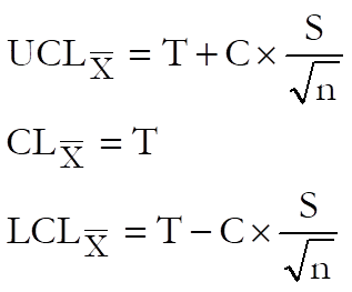
where:
· T is the target level. UNISTAT gives the overall mean of the samples as the default value. The weighted mean of the sample means.
· S is the sigma value. UNISTAT gives the overall sigma of the samples as the default value.
· C is control line parameter,
· n is the sample size.
Example
Table 7.2 on p. 192 from Banks, Jerry (1989). This is the continuation of the power socket manufacturing example in section 9.3.1.1. R Chart.
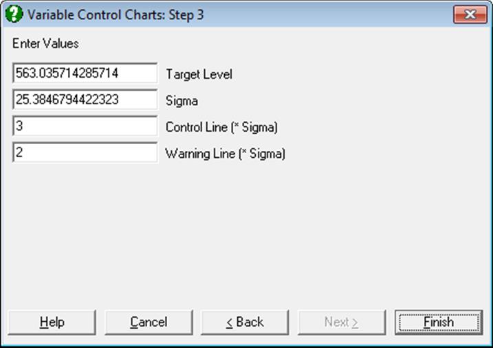
Open TIMESER and select Statistics 2 → Quality Control → Variable Control Charts. Select the data option 2 Enter Summary Data. Select X-Bar2 (C7) as [Mean] and R2 (C8) as [Range]. From the next dialogue select the sample size as 5. The variability is known to be under control, so select X Bar Chart at the next dialogue. The above data is continuation data from a process which has been under control previously, with calculated target levels (see example in 9.3.1.1. R Chart). So, at the next dialogue overwrite the default values with the following values which were obtained when the process was under control:
· 20.8185 Target Level
· 0.0116 Sigma
· 3 Control Line (* Sigma)
· 0 Warning Line (* Sigma)
· 0 MA Parameter (>1 MA, <1 EWMA)
· 0 Use Average N (0 No, Else Yes)
and from the final output dialogue click [Finish] to obtain the following chart:
Variable Control Charts
X Bar Chart
Size = 5.0000
Mean: X-bar2
Range: R2
‘*’ denotes sample outside control limits
|
Sample |
Value |
LCL |
UCL |
|
31/12/1899 Sun |
20.8180 |
20.8029 |
20.8341 |
|
01/01/1900 Mon |
20.8200 |
20.8029 |
20.8341 |
|
02/01/1900 Tue |
20.8210 |
20.8029 |
20.8341 |
|
03/01/1900 Wed |
20.8280 |
20.8029 |
20.8341 |
|
04/01/1900 Thu |
20.8250 |
20.8029 |
20.8341 |
|
05/01/1900 Fri |
20.8130 |
20.8029 |
20.8341 |
|
06/01/1900 Sat |
20.8280 |
20.8029 |
20.8341 |
|
07/01/1900 Sun |
20.8300 |
20.8029 |
20.8341 |
|
08/01/1900 Mon |
20.8320 |
20.8029 |
20.8341 |
|
* 09/01/1900 Tue |
20.8490 |
20.8029 |
20.8341 |
|
* 10/01/1900 Wed |
20.8480 |
20.8029 |
20.8341 |
|
* 11/01/1900 Thu |
20.8520 |
20.8029 |
20.8341 |
|
* 12/01/1900 Fri |
20.8420 |
20.8029 |
20.8341 |
|
* 13/01/1900 Sat |
20.8450 |
20.8029 |
20.8341 |
|
* 14/01/1900 Sun |
20.8410 |
20.8029 |
20.8341 |
|
Target Level = |
20.8185 |
|
Average Sample Size = |
5.0000 |
|
Control Limits = |
3.0000 x Sigma |
|
Sigma = |
0.0116 |
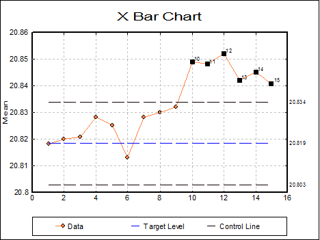
This shows that the process means are out of control. Since from the tenth sample onwards the points are above the UCL, the process must have gone out of control.
9.3.1.5. Moving Average Charts
Even if all the points lie inside the control lines on an X Bar Chart, this does not mean that the central tendency is under control. If a number of consecutive sample means all lie above the target level but under the control level, this may be an indication of a problem. The Moving Average Charts can be more sensitive than the standard X Bar Chart. The moving average of the sample means is plotted with the appropriate control lines. In UNISTAT two types of Moving Average Charts are available: (i) the standard moving average and (ii) the exponential weights moving average. The control lines for the two charts are quite different.
In these charts the moving average values of the sample means are plotted to control the central tendency of a variable. They will plot either standard moving average values or exponential weights moving average values. Both these charts assume the average sample size for all samples.
9.3.1.5.1. Standard Moving Average Charts
In this chart the standard moving average of the sample means are plotted to control the central tendency of a variable.
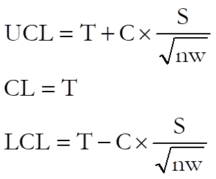
where:
· T is the target level. UNISTAT gives the overall mean of the samples as the default value. The weighted mean of the sample means.
· S is the sigma value. UNISTAT gives the overall sigma of the samples as the default value.
· C is the control line parameter,
· n is the sample size,
· w is the span of the moving average.
Example
Table 8.5 on p. 245 from Banks, Jerry (1989).
Open TIMESER and select Statistics 2 → Quality Control → Variable Control Charts. Select the data option 2 Enter Summary Data and Sample Size (C9) as [Size], X-Bar3 (C10) as [Mean] and Est Sigma (C11) as [Std Dev]. The variability is known to be under control, so select Moving Average Chart at the next dialogue. Next enter the following parameters:
· 10.1704545 Target Level
· 2.28 Sigma
· 3 Control Line (* Sigma)
· 0 Warning Line (* Sigma)
· 6 MA Parameter (>1 MA, <1 EWMA)
At the final output dialogue click [Next] to obtain the following chart:
Variable Control Charts
Moving Average Chart
Size: Sample Size
Mean: X-Bar3
Standard Deviation: Est Sigma
‘*’ denotes sample outside control limits
|
Sample |
Value |
LCL |
UCL |
|
31/12/1899 Sun |
10.2300 |
7.1115 |
13.2294 |
|
01/01/1900 Mon |
9.7250 |
8.0075 |
12.3335 |
|
02/01/1900 Tue |
9.9000 |
8.4044 |
11.9365 |
|
03/01/1900 Wed |
9.2900 |
8.6410 |
11.6999 |
|
04/01/1900 Thu |
9.3920 |
8.8025 |
11.5385 |
|
05/01/1900 Fri |
9.7600 |
8.9216 |
11.4193 |
|
06/01/1900 Sat |
9.9600 |
8.9216 |
11.4193 |
|
07/01/1900 Sun |
9.9117 |
8.9216 |
11.4193 |
|
08/01/1900 Mon |
10.0783 |
8.9216 |
11.4193 |
|
09/01/1900 Tue |
10.3950 |
8.9216 |
11.4193 |
|
10/01/1900 Wed |
10.7067 |
8.9216 |
11.4193 |
|
11/01/1900 Thu |
10.8250 |
8.9216 |
11.4193 |
|
12/01/1900 Fri |
10.8917 |
8.9216 |
11.4193 |
|
13/01/1900 Sat |
11.0383 |
8.9216 |
11.4193 |
|
14/01/1900 Sun |
10.9350 |
8.9216 |
11.4193 |
|
15/01/1900 Mon |
10.9967 |
8.9216 |
11.4193 |
|
16/01/1900 Tue |
10.7767 |
8.9216 |
11.4193 |
|
17/01/1900 Wed |
10.5050 |
8.9216 |
11.4193 |
|
18/01/1900 Thu |
10.2633 |
8.9216 |
11.4193 |
|
19/01/1900 Fri |
9.7800 |
8.9216 |
11.4193 |
|
20/01/1900 Sat |
9.5833 |
8.9216 |
11.4193 |
|
21/01/1900 Sun |
9.7067 |
8.9216 |
11.4193 |
|
Moving Average, N = |
6 |
|
Target Level = |
10.1705 |
|
Average Sample Size = |
5.0000 |
|
Control Limits = |
3.0000 x Sigma |
|
Sigma = |
2.2800 |
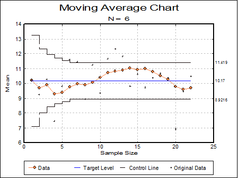
This chart shows that the process is in control.
9.3.1.5.2. Exponential Weights Moving Average Chart
This is sometimes called the geometric moving average control chart.
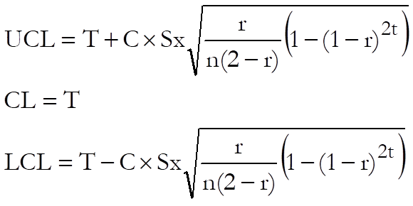
where:
· T is the target level. The default value is the overall mean of the samples, which is the weighted mean of the sample means.
· S is the sigma value. The default value is the overall sigma of the samples.
· C is the Control line parameter.
· n is the average sample size.
· r is the exponential weight parameter (1 ≤ r ≤ 0).
· t is the number of sample. This sequentially counts through the samples. It represents the number of samples which have contributed to the current moving average value.
Example
Table 8.6 on p. 249 from Banks, Jerry (1989).
Open TIMESER and select Statistics 2 → Quality Control → Variable Control Charts. Select the data option 2 Enter Summary Data and Sample Size (C9) as [Size], X-Bar3 (C10) as [Mean] and Est Sigma (C11) as [Std Dev]. The variability is known to be under control, so select Moving Average Chart at the next dialogue. Next enter the following parameters:
· 10.1704545 Target Level
· 2.28 Sigma
· 3 Control Line (* Sigma)
· 0 Warning Line (* Sigma)
· 0.25 Parameter (>1 MA, <1 EWMA)
and finally click [Finish] to obtain the following results:
Variable Control Charts
Moving Average Chart
Size: Sample Size
Mean: X-Bar3
Standard Deviation: Est Sigma
‘*’ denotes sample outside control limits
|
Sample |
Value |
LCL |
UCL |
|
31/12/1899 Sun |
10.1853 |
9.4057 |
10.9352 |
|
01/01/1900 Mon |
9.9440 |
9.2145 |
11.1264 |
|
02/01/1900 Tue |
10.0205 |
9.1222 |
11.2187 |
|
… |
… |
… |
… |
|
14/01/1900 Sun |
10.7737 |
9.0144 |
11.3265 |
|
15/01/1900 Mon |
10.5128 |
9.0143 |
11.3266 |
|
16/01/1900 Tue |
10.4721 |
9.0143 |
11.3266 |
|
17/01/1900 Wed |
10.5241 |
9.0143 |
11.3266 |
|
18/01/1900 Thu |
10.4881 |
9.0143 |
11.3266 |
|
19/01/1900 Fri |
9.5935 |
9.0143 |
11.3266 |
|
20/01/1900 Sat |
9.5577 |
9.0143 |
11.3266 |
|
21/01/1900 Sun |
9.7857 |
9.0143 |
11.3266 |
|
Moving Average, Lambda = |
0.2500 |
|
Target Level = |
10.1705 |
|
Average Sample Size = |
5.0000 |
|
Control Limits = |
3.0000 x Sigma |
|
Sigma = |
2.2800 |
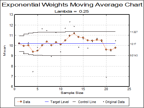
This chart shows that the process is in control.
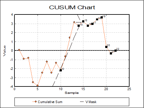
9.3.1.6. CUSUM Chart
The CUSUM Chart is used to control the central tendency, where the cumulative sum of differences from the target level is plotted. This means that even minor permanent shifts in the process will eventually lead to a sizeable cumulative sum of deviations.
The CUSUM Chart is completely different from other control charts because it has no control lines. Instead, a V-mask is used to control the variable, which is considered at each point in the series. If a previous point lies outside the V-mask the process is declared to be out of control.
Missing values are handled differently in CUSUM Charts, compared to the other control charts. To leave an empty column on the X-axis would affect the test of the V-mask. So, missing values are not drawn on the chart at all. This often results in the numbering on the X-axis looking somewhat strange.
The CUSUM Chart has the following input parameters:
Target Level: The target level is the centre line for the chart.
Sigma: The sigma value is the standard error of the variable.
Difference to Detect: This is the shift in the process mean to detect. Shifts less than this value are considered inconsequential. The value given is in terms of the standard deviation of each sample (sigma / average sample size).
Type I Error: The Type I error (alpha error) is the probability of declaring a process out of control when it is not.
Type II Error: The Type II error (beta error) is the probability of accepting a process is in control when it is out of control. A process is considered out of control when the mean shifts beyond the difference to detect.
Place V-Mask: This value allows the user to place the V-mask on any particular point in the data. If 0 is entered then the V-mask is placed on the first point where the chart is out of control. If the chart is in control then the V-mask is drawn on the last point in the series.
Example
Table 8.6 on p. 249 from Banks, Jerry (1989).
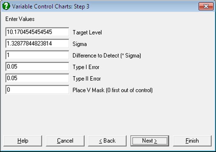
Open TIMESER and select Statistics 2 → Quality Control → Variable Control Charts. Select the data option 2 Enter Summary Data and Sample Size (C9) as [Size], X-Bar3 (C10) as [Mean] and Est Sigma (C11) as [Std Dev]. The variability is known to be under control, so select Cusum Chart at the next dialogue. Next enter the following parameters:
· 10.1704545 Target Level
· 2.28 Sigma
· 1 Difference to Detect (* Sigma)
· 0.05 Type I Error
· 0.05 Type II Error
· 0 Place V Mask (0 first out of control)
and finally click [Finish] to obtain the following results:
Variable Control Charts
CUSUM Chart
Size: Sample Size
Mean: X-Bar3
Standard Deviation: Est Sigma
‘*’ denotes sample outside V Mask at 13
|
Sample |
Value |
V Mask Upper |
V Mask Lower |
|
31/12/1899 Sun |
0.0595 |
-12.2146 |
18.4628 |
|
01/01/1900 Mon |
-0.8909 |
-11.0746 |
17.3228 |
|
02/01/1900 Tue |
-0.8114 |
-9.9346 |
16.1828 |
|
03/01/1900 Wed |
-3.5218 |
-8.7946 |
15.0428 |
|
04/01/1900 Thu |
-3.8923 |
-7.6546 |
13.9028 |
|
05/01/1900 Fri |
-2.4627 |
-6.5146 |
12.7628 |
|
06/01/1900 Sat |
-1.2032 |
-5.3746 |
11.6228 |
|
07/01/1900 Sun |
-2.4436 |
-4.2346 |
10.4828 |
|
08/01/1900 Mon |
-1.3641 |
-3.0946 |
9.3428 |
|
* 09/01/1900 Tue |
-2.1745 |
-1.9546 |
8.2028 |
|
10/01/1900 Wed |
-0.6750 |
-0.8146 |
7.0628 |
|
11/01/1900 Thu |
1.4645 |
0.3254 |
5.9228 |
|
12/01/1900 Fri |
3.1241 |
1.4654 |
4.7828 |
|
* 13/01/1900 Sat |
2.7636 |
-1.0000e+030 |
1.0000e+030 |
|
* 14/01/1900 Sun |
3.2232 |
-1.0000e+030 |
1.0000e+030 |
|
* 15/01/1900 Mon |
2.7827 |
-1.0000e+030 |
1.0000e+030 |
|
* 16/01/1900 Tue |
2.9623 |
-1.0000e+030 |
1.0000e+030 |
|
* 17/01/1900 Wed |
3.4718 |
-1.0000e+030 |
1.0000e+030 |
|
* 18/01/1900 Thu |
3.6814 |
-1.0000e+030 |
1.0000e+030 |
|
* 19/01/1900 Fri |
0.4209 |
-1.0000e+030 |
1.0000e+030 |
|
* 20/01/1900 Sat |
-0.2995 |
-1.0000e+030 |
1.0000e+030 |
|
* 21/01/1900 Sun |
0.0000 |
-1.0000e+030 |
1.0000e+030 |
|
Target Level = |
10.1705 |
|
Average Sample Size = |
5.0000 |
|
Sigma = |
2.2800 |
|
Difference to Detect = |
1.0000 x Sigma |
|
Type I Error = |
0.0500 |
|
Type II Error = |
0.0500 |
9.3.1.7. Table of Values
For each sample, the sample sizes, means, standard deviations and ranges are displayed in a table. These values can be saved to the data matrix and used as input to Variable Control Charts.
Example
Table 7.5 on p. 214 from Banks, Jerry (1989). Refractive Index of Fiber Optic Cable is given.
Open TIMESER and select Statistics 2 → Quality Control → Variable Control Charts. Select the data option 1 Enter Raw Values and Samples and Day (C5) as [Sample] and Refractive Index (C6) as [Variable]. From the next dialogue select Table of Values to obtain the following results:
Variable Control Charts
Table of Values
|
Sample |
Size |
Mean |
Standard Deviation |
Range |
|
08/06/1992 Mon |
6 |
95.7333 |
1.1466 |
3.2000 |
|
09/06/1992 Tue |
6 |
95.4667 |
1.2501 |
3.7000 |
|
10/06/1992 Wed |
4 |
96.6500 |
1.5948 |
3.2000 |
|
11/06/1992 Thu |
5 |
97.4600 |
0.8204 |
1.9000 |
|
12/06/1992 Fri |
6 |
96.8667 |
1.5870 |
3.8000 |
|
15/06/1992 Mon |
4 |
96.8500 |
1.4617 |
3.5000 |
|
16/06/1992 Tue |
8 |
96.5250 |
1.3307 |
3.4000 |
|
17/06/1992 Wed |
4 |
96.0750 |
1.0996 |
2.3000 |
|
18/06/1992 Thu |
6 |
97.2333 |
1.4828 |
4.4000 |
|
19/06/1992 Fri |
5 |
96.5400 |
0.8019 |
1.9000 |
|
22/06/1992 Mon |
6 |
96.6333 |
1.4166 |
4.0000 |
|
23/06/1992 Tue |
5 |
96.4600 |
0.7668 |
1.8000 |
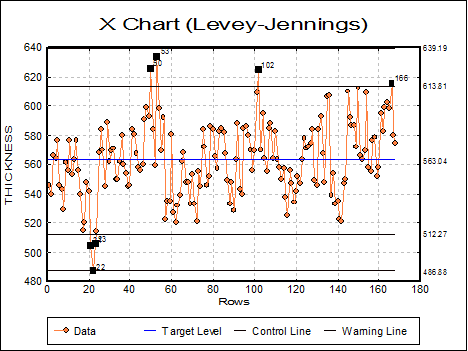
9.3.1.8. X Chart (Levey-Jennings)
This is a simple X-Y plot with the ability to display target and control lines and mark and annotate outlying points.
Variable selection is similar to that of other Variable Control Charts (see 9.3.0.2. Control Chart Inputs). A data column containing control measurements is selected clicking on [Variable] and a categorical data column (containing string or numeric values) is selected by clicking on [Sample]. The latter will not affect the appearance of the curve, but it can be used to label the group membership of outlying points (see 9.3.1.0.1. Raw Values and Samples).
The parameter input dialogue displays the mean and standard deviation as calculated from data. Also displayed are the levels of warning and control lines as multiples of sigma. Here, you can either accept these values or enter other values.
By default, all points are plotted without annotation. It is possible, however, to select Edit → Data Series and display case labels for outlying values.
Example
Open TIMESER and select Statistics 2 → Quality Control → Variable Control Charts. From the Variable Selection Dialogue select THICKNESS (C21) as [Variable] and ZONE (C19) as [Factor]. On Step 2 select X Chart (Levey-Jennings) and on the next step enter 2 for Warning Line (* Sigma).