6.4.1. Unpaired Samples
Data in one of the three types supported for Two Sample Tests can be used for these tests. Missing values are omitted by case.
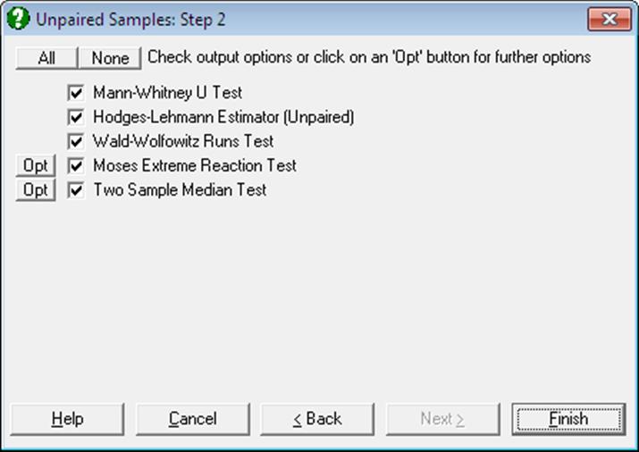
Moses Extreme Reaction Test and Two Sample Median Test have a further dialogue each, which can be accessed by clicking on their [Opt] buttons situated to the left of the check boxes. If [Finish] is clicked before [Opt], then the program will use the default values suggested by the program, without displaying their further dialogues.
6.4.1.1. Mann-Whitney U Test
This test is used to determine whether two independent random samples have been drawn from the same population. The null hypothesis tested is that “the population relative frequency distributions are identical” against the alternative hypothesis that “they are different” (two-tailed test).
The output includes the number of cases, rank sums, mean ranks, and U scores for the two samples as well as the test statistic, correction for ties and the asymptotic (normal and t-) and exact two-tailed probability values, with and without continuity correction.
The test statistic U for sample 1 is obtained by summing the number of times cases in sample 1 are smaller than cases in sample 2. U for sample 2 is found similarly. The smaller U value is chosen as the test statistic. A small or large U value indicates that the two samples are not similarly distributed. U values can also be calculated as:
U1 = n1n2 + n1(n1+1)/2 – R1
U2 = n1n2 + n2(n2+1)/2 – R2
where R1 and R2 are the sum of ranks for groups 1 and 2 respectively.
The program will compute and display a Z statistic which is corrected for ties and with no continuity correction as:
![]()
where the mean of the Mann-Whitney distribution is given as:
![]()
and its standard deviation as:
![]()
where:
n = n1 + n2
and wi1 is the rank of the ith case belonging to group 1, supposing that group 1 has the smaller U.
The Z statistic with continuity correction is:
![]()
One- and two-tailed probabilities from normal and t-distributions (with n – 1 degrees of freedom) are displayed for Z-statistic without and with continuity correction.
The following alternative definition of the standard deviation (given by Armitage & Berry (2002) p. 276 and Gardner & Altman (2000) p. 40) is not used here as it does not take ties into consideration:
![]()
An exact p-value is also computed which is accurate for data sets with or without ties. By default, it is reported for n £ 150, though this limit can be changed by the user. To do this, the following line should be entered and edited in the [Options] section of Documents\Unistat10\Unistat10.ini file:
WMWMaxExactSize=150
This limit can be extended if there are no ties in data. However, if ties exist, the exact p-value for n > 150 may take a long time to compute.
It is also possible to save the complete exact one-tailed cumulative probability distribution of the test statistic in its rank sum form by including the following line in the [Options] section of Unistat10.ini:
WMWSaveDist=1
By default, the distribution will be saved to the following file:
Documents\Unistat10\WMWExactDist.txt
This file name can be changed by entering and editing the following line in the [Options] section of Unistat10.ini:
WMWSaveDistFile=..\Documents\Unistat10\WMWExactDist.txt
Example 1
Example 10.3 on p. 279 from Armitage & Berry (2002). An estimate of the median difference is required. A comparison of 32 inpatients and 32 outpatients is made.
Open NONPAR12 and select Statistics 1 → Nonparametric Tests (1-2 Samples) → Unpaired Samples. Select Inpatients (C16) and Outpatients (C17) as [Variable]s and check only the Mann-Whitney U Test output option to obtain the following results:
Unpaired Samples
Mann-Whitney U Test
|
|
Cases |
Rank Sum |
Mean Rank |
U |
|
Inpatients |
32 |
858.0000 |
26.8125 |
694.0000 |
|
Outpatients |
32 |
1222.0000 |
38.1875 |
330.0000 |
|
Total |
64 |
2080.0000 |
32.5000 |
|
|
Correction for Ties = |
410.5000 |
|
|
U |
Test Statistic |
1-Tail Probability |
2-Tail Probability |
|
Asymptotic Normal |
330.0000 |
-2.4670 |
0.0068 |
0.0136 |
|
Asymptotic Normal with CC |
|
-2.4603 |
0.0069 |
0.0139 |
|
Asymptotic t |
|
-2.4670 |
0.0082 |
0.0164 |
|
Asymptotic t with CC |
|
-2.4603 |
0.0083 |
0.0166 |
|
Exact |
|
|
0.0065 |
0.0131 |
It is concluded that the medians of the two samples are significantly different. A t-test cannot detect a significant difference between the two sample means. This example shows the power of Mann-Whitney U Test when the assumption of normality fails.
Example 2
Example 8.11 on p. 164 from Zar, J. H. (2010). The null hypothesis “there is no difference between the heights of male and female students” is tested.
Open NONPAR12 and select Statistics 1 → Nonparametric Tests (1-2 Samples) → Unpaired Samples. Select Males (C18) and Females (C19) as [Variable]s and check only the Mann-Whitney U Test output option to obtain the following results:
Unpaired Samples
Mann-Whitney U Test
|
|
Cases |
Rank Sum |
Mean Rank |
U |
|
Males |
7 |
60.0000 |
8.5714 |
3.0000 |
|
Females |
5 |
18.0000 |
3.6000 |
32.0000 |
|
Total |
12 |
78.0000 |
6.5000 |
|
|
Correction for Ties = |
0.0000 |
|
|
U |
Test Statistic |
1-Tail Probability |
2-Tail Probability |
|
Asymptotic Normal |
3.0000 |
-2.3548 |
0.0093 |
0.0185 |
|
Asymptotic Normal with CC |
|
-2.2736 |
0.0115 |
0.0230 |
|
Asymptotic t |
|
-2.3548 |
0.0191 |
0.0382 |
|
Asymptotic t with CC |
|
-2.2736 |
0.0220 |
0.0440 |
|
Exact |
|
|
0.0088 |
0.0177 |
Zar reports the exact two-tailed probability as 0.018 and since this is less than 0.05, we reject the null hypothesis.
If the WMWSaveDist=1 line is included in the [Options] section of Documents\Unistat10\Unistat10.ini file, the exact one-tailed cumulative distribution of the rank sum is saved to the WMWExactDist.txt file as follows:
|
Rank Sum |
One Tail Probability |
|
|
|
|
28 |
1.26262626262626E-03 |
|
46 |
0.561868686868687 |
|
29 |
2.52525252525253E-03 |
|
47 |
0.622474747474747 |
|
30 |
5.05050505050505E-03 |
|
48 |
0.680555555555555 |
|
31 |
8.83838383838384E-03 |
|
49 |
0.734848484848485 |
|
32 |
1.51515151515152E-02 |
|
50 |
0.784090909090909 |
|
33 |
0.023989898989899 |
|
51 |
0.828282828282828 |
|
34 |
3.66161616161616E-02 |
|
52 |
0.866161616161616 |
|
35 |
0.053030303030303 |
|
53 |
0.898989898989899 |
|
36 |
7.44949494949495E-02 |
|
54 |
0.92550505050505 |
|
37 |
0.101010101010101 |
|
55 |
0.946969696969697 |
|
38 |
0.133838383838384 |
|
56 |
0.963383838383838 |
|
39 |
0.171717171717172 |
|
57 |
0.976010101010101 |
|
40 |
0.215909090909091 |
|
58 |
0.984848484848485 |
|
41 |
0.265151515151515 |
|
59 |
0.991161616161616 |
|
42 |
0.319444444444444 |
|
60 |
0.994949494949495 |
|
43 |
0.377525252525252 |
|
61 |
0.997474747474747 |
|
44 |
0.438131313131313 |
|
62 |
0.998737373737374 |
|
45 |
0.5 |
|
63 |
1 |
6.4.1.2. Hodges-Lehmann Estimator (Unpaired)
If the product of the two sample sizes does not exceed 2 x 10⁹ then an estimate of the difference between the two sample medians and its confidence interval are computed.
First, all n1 x n2 differences between each pair of numbers from the two samples are sorted in increasing order. Then, the median (the Hodges-Lehmann estimator or the shift parameter) is found.
The output includes a table where the minimum, maximum, mean and standard deviation of the rank sum are displayed. The mean of the rank sum is different from the mean of the Mann-Whitney statistic, whereas their standard deviations are the same.
The limits of the asymptotic confidence interval are the Kth smallest and the Kth largest difference:
![]()
where K is rounded up to the nearest integer and the mean and standard deviation of the Mann-Whitney statistic are as given in the previous section.
The exact confidence interval is also displayed, which is based on the exact distribution of the Mann-Whitney statistic. To determine the lower bound of the exact interval (the Klth smallest difference), find kl such that:
![]()
round kl up to the nearest integer and calculate:
![]()
The upper limit is determined likewise, for:
![]() .
.
For the paired case of this test see 6.4.2.2. Hodges-Lehmann Estimator (Paired).
Example 1
Example 10.4 on p. 283 from Armitage & Berry (2002). Gain in weight of rats receiving diets with high and low protein content are measured. The null hypothesis “there is no difference in median weights” is tested at 95% level.
Open NONPAR12 and select Statistics 1 → Nonparametric Tests (1-2 Samples) → Unpaired Samples. Select High (C1) and Low (C2) as [Variable]s and check the Hodges-Lehmann Estimator (Unpaired) output option to obtain the following results:
Unpaired Samples
Hodges-Lehmann Estimator (Unpaired)
For High and Low
|
|
Minimum |
Maximum |
Mean |
Standard Deviation |
|
Rank Sum |
78.0000 |
162.0000 |
120.0000 |
11.8270 |
|
|
K |
Difference Between Medians |
Lower 95% |
Upper 95% |
|
Asymptotic |
19 |
18.5000 |
-3.0000 |
40.0000 |
|
Exact |
|
|
-3.0000 |
40.0000 |
6.4.1.3. Wald-Wolfowitz Runs Test
The null hypothesis “two independent samples have been drawn from the same population” is tested against the alternative hypothesis “they differ in respect of their medians, variability or skewness”. It is assumed that the variable under consideration has a continuous distribution.
All cases from the two samples are sorted together. If the two distributions are similar, then cases belonging to two samples must be scattered randomly. Then the program counts the number of runs (i.e. the number of groups of cases which belong to the same sample). If there are ties between cases belonging to two samples then the minimum and the maximum possible number of runs are reported separately. Two sets of results using the normal approximation are reported.
Asymptotic without Continuity Correction: In this case the Z-statistic is defined as:
![]()
where:
![]()
![]()
Asymptotic with Continuity Correction: The Z-statistic with continuity correction is defined as:
![]()
In some applications, the test statistic with
continuity correction is reported for ![]() and
without continuity correction otherwise. The same normal approximation is also used for the Runs Test.
and
without continuity correction otherwise. The same normal approximation is also used for the Runs Test.
Exact: The exact one- and two-tailed probabilities are reported. Their use is recommended for n £ 30.
Data in one of the three types supported for Two Sample Tests can be used for this test. Missing values are omitted by case.
Example
Table 100 on p. 251 from Cohen, L. & M. Holliday (1983). Aggression scores in 20 nursery school children following violent (Condition 1) and neutral (Condition 0) cartoons are given.
Open NONPAR12 and select Statistics 1 → Nonparametric Tests (1-2 Samples) → Unpaired Samples. Select Score (C13) as [Variable] and Condition (C14) as [Factor]. From the next dialogue uncheck the Run a separate analysis for each option selected box and select only the Wald-Wolfowitz Runs Test option:
Unpaired Samples
Wald-Wolfowitz Runs Test
Data variable: Score
Subsample selected by: Condition
|
Condition |
Cases |
Mean |
Standard Deviation |
Standard Error |
|
0 |
10 |
24.2000 |
19.5209 |
6.1731 |
|
1 |
10 |
46.2000 |
14.1327 |
4.4692 |
|
Total |
20 |
35.2000 |
17.0411 |
3.8105 |
|
|
Number of Runs |
Z-Statistic |
1-Tail Probability |
2-Tail Probability |
|
Asymptotic |
8 |
-1.3784 |
0.0840 |
0.1681 |
|
Asymptotic with CC |
|
-1.1487 |
0.1253 |
0.2507 |
|
Exact |
|
|
0.1276 |
|
This result is not significant at the 10% level. Hence do not reject the null hypothesis “watching violent cartoons does not cause a significant change in the aggression of nursery school children”.
6.4.1.4. Moses Extreme Reaction Test
This test is used to determine the difference in range between two samples. Cases from the two samples are ranked together. Ranks corresponding to the smallest and largest group 1 cases are determined. The span is the difference between these two ranks plus one.
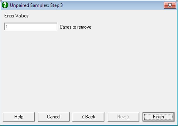
The program will prompt for the number of cases to be trimmed from either side of the span. The suggested number is either 1 or the integer closest to 5% of the number of cases in group 1, whichever is larger. However, this number can be changed by the user. The output includes the number of cases in two groups as well as the span and the one-tailed probability.
The exact one-tailed probability is computed for n £ 150. This limit can be changed by entering the following line with the appropriate number in the [Options] section of Documents\Unistat10\Unistat10.ini file:
WMWMaxExactSize=150
Example
Open DEMODATA and select Statistics 1 → Nonparametric Tests (1-2 Samples) → Unpaired Samples. Select Wages (C2) and Energy (C3) as [Variable]s and click on the [Opt] button next to the Moses Extreme Reaction Test option. Accept the default value of 3 from the next dialogue.
Unpaired Samples
Moses Extreme Reaction Test
|
|
Cases |
|
Wages |
57 |
|
Energy |
57 |
|
Total |
114 |
|
|
span |
1-Tail Probability |
|
whole of group 1 |
108 |
0.0567 |
|
3 case(s) removed from ends |
92 |
0.0302 |
6.4.1.5. Two Sample Median Test
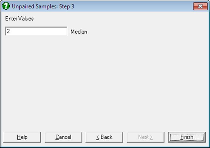
This test is used to determine whether two samples are drawn from populations with similar medians. The median for the two combined samples is calculated, the two samples are dichotomised and a 2 x 2 table is formed. It is possible to edit the computed median and to enter any values. The output includes the generated 2 x 2 table, chi square test statistics without and with a continuity correction and the exact probabilities.
Asymptotic without Continuity Correction: The following chi-square statistic with one degree of freedom is compared with the chi-square distribution:
![]()
Asymptotic with Continuity Correction: In this case the numerator is slightly different:
![]()
where g1 and g2 are the number of cases greater than the median in samples 1 and 2 respectively.
Exact: Two-tailed and table probabilities are reported using Fisher’s exact probability formula (see 6.4.5.2. Fisher’s Exact Test).
Example
Example 8.18 on p. 156 from Zar, J. H. (1999). The null hypothesis “the medians of the two sampled populations are equal” is tested.
Open NONPAR12 and select Statistics 1 → Nonparametric Tests (1-2 Samples) → Unpaired Samples and select Assistant A (C20) and Assistant B (C21) as [Variable]s. Note that these are the rank data in descending order. Select the Two Sample Median Test output option to obtain the following results:
Unpaired Samples
Two Sample Median Test
|
|
> Median |
<=Median |
Total |
|
Assistant A |
6 |
5 |
11 |
|
Assistant B |
6 |
8 |
14 |
|
Total |
12 |
13 |
25 |
|
|
Median |
Chi-Square Statistic |
Degrees of Freedom |
Right-Tail Probability |
|
Asymptotic |
12.5000 |
0.3372 |
1 |
0.5615 |
|
Asymptotic with CC |
|
0.0315 |
1 |
0.8592 |
|
|
2-Tail Probability |
Table Probability |
|
Fisher’s Exact |
0.6951 |
0.2668 |
Since P > 0.05, do not reject the null hypothesis. In the 5th edition of Biostatistical Analysis (2010) Example 8.15 on p. 173, Zar employs a different method where observations at the median are omitted. With this approach the total number of valid cases is 23 and the chi-squared statistic with continuity correction is 0.473.