6.4.2. Paired Samples
Like the nonparametric tests on unpaired samples of the previous section, the tests in this section are also used to assess the significance of the difference between population distributions of two samples. In this case the two samples are assumed to consist of matched pairs.
In general, a test is run on paired data by selecting two numeric data columns as [Variable]s. When three or more columns are selected the test will be performed on all possible pairs with equal length (see 6.0.3. Tests with Paired Data). The missing values are omitted pairwise.
Despite the section title Paired Samples, it is also possible to select a single column. When only one column is selected, the test is performed against a hypothetical second variable consisting of zeros.
An Output Options Dialogue offering four options is displayed next.
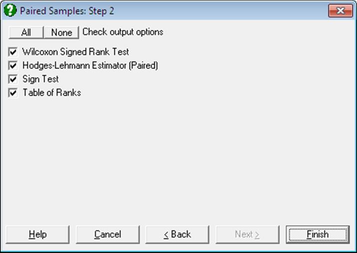
6.4.2.1. Wilcoxon Signed Rank Test
This test is used to assess the significance of the difference between population distributions of the two samples consisting of matched pairs. The absolute values of the difference between the pairs are ranked and the rank sums of negative and positive differences are computed. The signed ranks can be displayed using the Table of Ranks option below.
A very small or a very large sum indicates that the two samples do not have similar distributions. The smaller of the two values is selected as the test statistic.
Missing values are omitted pairwise. The output includes a table displaying the number of positive and negative differences, rank sums and mean ranks. One- and two-tailed asymptotic probabilities are reported without and with continuity correction, as well as the one- and two-tailed exact probabilities.
Asymptotic without Continuity Correction: The Z-statistic is defined as:
![]()
Asymptotic with Continuity Correction: In this case the Z-statistic is:
![]()
where the mean of the Wilcoxon Signed Rank distribution is given as:
![]()
and its standard deviation:
![]()
R is the smaller sum of the like-signed ranks (the test statistic) and T is the sum of t3 – t where t is the number of ties at a given rank.
If n > 20 then the Z statistic provides a good approximation for the distribution of the test statistic. The exact p-value is reported for n £ 150 and it is accurate for data sets with or without ties. To change this limit, the following line should be entered and edited in the [Options] section of Documents\Unistat10\Unistat10.ini file:
WMWMaxExactSize=150
It is also possible to save the complete exact one-tailed cumulative probability distribution of the test statistic by including the following line in the [Options] section of Unistat10.ini:
WMWSaveDist=1
By default, the distribution will be saved to the following file:
..\Documents\Unistat10\WMWExactDist.txt
This file name can be changed by entering and editing the following line in the [Options] section of Documents\Unistat10\Unistat10.ini file:
WMWSaveDistFile=..\Documents\Unistat10\WMWExactDist.txt
Example 1
Example 10.2 on p. 275 from Armitage & Berry (2002). The null hypothesis “there is no difference between the effects of the drug and the placebo” is tested.
Open NONPAR12 and select Statistics 1 → Nonparametric Tests (1-2 Samples) → Paired Samples. Select Drug (C5) and Placebo (C6) as [Variable]s and check only the Wilcoxon Signed Rank Test output option to obtain the following results:
Paired Samples
Wilcoxon Signed Rank Test
For Drug and Placebo
|
|
Cases |
Rank Sum |
Mean Rank |
|
Negative Differences |
6 |
38.0000 |
6.3333 |
|
Positive Differences |
4 |
17.0000 |
4.2500 |
|
Total |
10 |
55.0000 |
5.5000 |
|
Correction for Ties = |
1.5000 |
|
|
W |
Z-Statistic |
1-Tail Probability |
2-Tail Probability |
|
Asymptotic |
17.0000 |
-1.0273 |
0.1521 |
0.3043 |
|
Asymptotic with CC |
|
-1.0787 |
0.1404 |
0.2807 |
|
Exact |
|
|
0.1611 |
0.3223 |
Since the two-tailed probability is far greater than 5% the test result is not significant. Therefore, do not reject the null hypothesis.
If the WMWSaveDist=1 line is included in the [Options] section of Documents\Unistat10\Unistat10.ini file, the exact one-tailed cumulative distribution of the rank sum is saved to the WMWExactDist.txt file as follows (shortened):
|
Rank Sum |
One Tail Probability |
|
|
|
|
0 |
0.0009765625 |
|
… |
… |
|
2.5 |
0.0048828125 |
|
42 |
0.931640625 |
|
5 |
0.01171875 |
|
42.5 |
0.935546875 |
|
6.5 |
0.013671875 |
|
43 |
0.943359375 |
|
7.5 |
0.021484375 |
|
43.5 |
0.95703125 |
|
8 |
0.0224609375 |
|
44.5 |
0.9609375 |
|
9 |
0.0302734375 |
|
45 |
0.9677734375 |
|
9.5 |
0.0322265625 |
|
45.5 |
0.9697265625 |
|
10 |
0.0390625 |
|
46 |
0.9775390625 |
|
10.5 |
0.04296875 |
|
47 |
0.978515625 |
|
11.5 |
0.056640625 |
|
47.5 |
0.986328125 |
|
12 |
0.064453125 |
|
48.5 |
0.98828125 |
|
12.5 |
0.068359375 |
|
50 |
0.9951171875 |
|
13 |
0.076171875 |
|
52.5 |
0.9990234375 |
|
… |
… |
|
55 |
1 |
Example 2
Example 9.4, p. 185 from Zar, J. H. (2010). The null hypothesis “deer hindleg length is the same as foreleg length” is tested.
Open NONPAR12 and select Statistics 1 → Nonparametric Tests (1-2 Samples) → Paired Samples. Select Hindleg (C7) and Foreleg (C8) as [Variable]s and check only the Wilcoxon Signed Rank Test output option to obtain the following results:
Paired Samples
Wilcoxon Signed Rank Test
For Hindleg and Foreleg
|
|
Cases |
Rank Sum |
Mean Rank |
|
Negative Differences |
2 |
4.0000 |
2.0000 |
|
Positive Differences |
8 |
51.0000 |
6.3750 |
|
Total |
10 |
55.0000 |
5.5000 |
|
Correction for Ties = |
0.7500 |
|
|
W |
Z-Statistic |
1-Tail Probability |
2-Tail Probability |
|
Asymptotic |
4.0000 |
-2.3536 |
0.0093 |
0.0186 |
|
Asymptotic with CC |
|
-2.4047 |
0.0081 |
0.0162 |
|
Exact |
|
|
0.0059 |
0.0117 |
Since the probability is less than 5%, reject the null hypothesis.
6.4.2.2. Hodges-Lehmann Estimator (Paired)
This statistic will estimate the median difference. First, the difference between each pair is computed for n cases. Then the averages of all combinations of differences (also known as Walsh averages) are computed. The n(n + 1)/2 averages are sorted in increasing order and their median (the Hodges-Lehmann estimator or the shift parameter) is found.
The output includes a table where the minimum, maximum, mean and standard deviation of the test statistic are displayed.
The limits of the asymptotic confidence interval are the K*th smallest and the K*th largest difference:
![]()
where K* is rounded up to the nearest integer and the mean and standard deviation of the signed rank statistic are as given in the previous section.
The exact confidence interval is also displayed, which is based on the exact distribution of the test statistic. To determine the lower bound of the exact interval (the K*l smallest difference), find K*l such that:
![]()
round K*l up to the nearest integer. The upper limit is determined likewise, for:
![]()
For the unpaired case of this test see 6.4.1.2. Hodges-Lehmann Estimator (Unpaired).
Example 1
Example 10.2 on p. 276 from Armitage & Berry (2002). An estimate of the median difference is required.
Open NONPAR12 and select Statistics 1 → Nonparametric Tests (1-2 Samples) → Paired Samples. Select Drug (C5) and Placebo (C6) as [Variable]s and check only the Hodges-Lehmann Estimator (Paired) output option to obtain the following results:
Paired Samples
Hodges-Lehmann Estimator (Paired)
For Drug and Placebo
|
|
Minimum |
Maximum |
Mean |
Standard Deviation |
|
Rank Sum |
0.0000 |
55.0000 |
27.5000 |
9.7340 |
|
|
K* |
Median of Walsh Differences |
Lower 95% |
Upper 95% |
|
Asymptotic |
9 |
-1.0000 |
-4.5000 |
1.0000 |
|
Exact |
|
|
-4.5000 |
1.0000 |
Example 2
Table 5.3 on p. 42, Gardner & Altman (2000). Beta endorphin concentrations in subjects before and after running in a half marathon are measured. We would like to estimate the sample median for the pairwise averages between differences and the 95% confidence intervals.
Open NONPAR12 and select Statistics 1 → Nonparametric Tests (1-2 Samples) → Paired Samples. Select After (C9) and Before (C10) as [Variable]s and check only the Hodges-Lehmann Estimator (Paired) output option to obtain the following results:
Paired Samples
Hodges-Lehmann Estimator (Paired)
For After and Before
|
|
Minimum |
Maximum |
Mean |
Standard Deviation |
|
Rank Sum |
0.0000 |
66.0000 |
33.0000 |
11.2472 |
|
|
K* |
Median of Walsh Differences |
Lower 95% |
Upper 95% |
|
Asymptotic |
11 |
18.8250 |
11.9000 |
25.1000 |
|
Exact |
|
|
11.9000 |
25.1000 |
6.4.2.3. Sign Test
This is a weaker version of Wilcoxon Signed Rank Test. The negative and positive differences are counted and the ties are ignored. Since the probability that either sum exceeds the other is 0.5, it is equivalent to a Binomial Test with p = 0.5.
The exact probability is calculated from the binomial distribution. The asymptotic probability is based on a normal approximation:
![]()
where np and nn are the numbers of positive and negative differences respectively. In both cases a two-tailed probability is reported. The output consists of the number of negative and positive differences, number of ties, test statistic and the exact binomial and asymptotic two-tailed probabilities.
Example 1
Example 10.1 on p. 274 from Armitage & Berry (2002). The null hypothesis “there is no difference between the effects of the drug and the placebo” is tested.
Open NONPAR12 and select Statistics 1 → Nonparametric Tests (1-2 Samples) → Paired Samples. Select Drug (C5) and Placebo (C6) as [Variable]s and check only the Sign Test output option to obtain the following results:
Paired Samples
Sign Test
For Drug and Placebo
|
|
Cases |
|
Negative Differences |
6 |
|
Positive Differences |
4 |
|
Ties |
0 |
|
Total |
10 |
|
|
Value |
Z-Statistic |
1-Tail Probability |
2-Tail Probability |
|
Asymptotic |
6.0000 |
0.3162 |
0.3759 |
0.7518 |
|
Exact |
|
|
0.3770 |
0.7539 |
Example 2
Example 24.10, p. 538 from Zar, J. H. (2010). The null hypothesis is “deer hindleg length is the same as foreleg length”.
Open NONPAR12 and select Statistics 1 → Nonparametric Tests (1-2 Samples) → Paired Samples. Select Hindleg (C7) and Foreleg (C8) as [Variable]s and check only the Sign Test output option to obtain the following results:
Paired Samples
Sign Test
For Hindleg and Foreleg
|
|
Cases |
|
Negative Differences |
2 |
|
Positive Differences |
8 |
|
Ties |
0 |
|
Total |
10 |
|
|
Value |
Z-Statistic |
1-Tail Probability |
2-Tail Probability |
|
Asymptotic |
8.0000 |
1.5811 |
0.0569 |
0.1138 |
|
Exact |
|
|
0.0547 |
0.1094 |
Since the two-tailed exact binomial probability is greater than 5%, do not reject the null hypothesis.
6.4.2.4. Table of Ranks
When this output option is selected, a table will be formed displaying the two columns, their differences, the signed rank of their absolute value and the differences ordered in ascending order. The signed ranks are the intermediate values used in Wilcoxon Signed Rank Test.
The last column, ordered difference, can be used to run a Walsh Test. This test is used to determine whether two samples have been drawn from symmetrically distributed populations. It is assumed that the distributions are continuous. The test can be performed meaningfully only on small data sets with n £ 15.
First the signed difference for each matched pair is computed and then differences are ranked in increasing size. The null hypothesis is that “the average of differences is equal to zero” against the alternative hypothesis that “the population mean is other than zero”. Output displays the two data columns, their differences and the ranked difference. For probability values, tables for the Walsh Test must be consulted.
Example
Table 99 on p. 248 from Cohen, L. & M. Holliday (1983). With and without practice errors in a manual dexterity selection test are given for 11 candidates.
Open NONPAR12 and select Statistics 1 → Nonparametric Tests (1-2 Samples) → Paired Samples. Select Without (C11) and With (C12) as [Variable]s and check only the Table of Ranks output option to obtain the following results:
Paired Samples
Table of Ranks
For Without and With
|
Row |
Without |
With |
Difference |
Signed Rank |
Ordered Difference |
|
1 |
11.0000 |
6.0000 |
5.0000 |
7.5000 |
-1.0000 |
|
2 |
4.0000 |
2.0000 |
2.0000 |
3.0000 |
0.0000 |
|
3 |
5.0000 |
4.0000 |
1.0000 |
1.5000 |
1.0000 |
|
4 |
9.0000 |
3.0000 |
6.0000 |
9.5000 |
2.0000 |
|
5 |
5.0000 |
5.0000 |
0.0000 |
0.0000 |
3.0000 |
|
6 |
13.0000 |
7.0000 |
6.0000 |
9.5000 |
4.0000 |
|
7 |
5.0000 |
6.0000 |
-1.0000 |
-1.5000 |
4.0000 |
|
8 |
7.0000 |
3.0000 |
4.0000 |
5.5000 |
5.0000 |
|
9 |
8.0000 |
4.0000 |
4.0000 |
5.5000 |
5.0000 |
|
10 |
10.0000 |
7.0000 |
3.0000 |
4.0000 |
6.0000 |
|
11 |
12.0000 |
7.0000 |
5.0000 |
7.5000 |
6.0000 |
Consult tables for critical values of the Walsh Test with n = 11. We see from the table that a two-tailed test with n =11 is significant at the 5.6% level if:
max[d7, ½(d5+d11)] < 0 or min[d5, ½(d1+d7)] > 0
In this example:
max[4, ½(3+6)] < 0 or min[3, ½(-1+4)] > 0
max[4, 4½] < 0 or min[3, 2½] > 0
Since 3 > 0, this result is significant at the 5.6% level. Hence reject the null hypothesis that “manual dexterity does not change with practice”.