8.1.1. Hierarchical Cluster Analysis
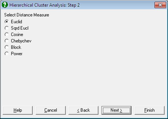
First, select the data columns to be analysed by clicking on [Variable] from the Variable Selection Dialogue. If the data is not a proximity matrix (if it is not square and symmetric) then another dialogue will appear allowing you to choose from six distance measures. This dialogue will not be available when you input a proximity matrix.
8.1.1.1. Distance Measures
Euclid:
![]()
Squared Euclid:
![]()
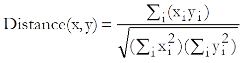
Cosine:
Chebychev:
![]()
Block:
![]()
Power:
![]()
where the power terms p and r are supplied by the user.
8.1.1.2. Distance Matrix
After the distance matrix is computed, a dialogue containing nine hierarchical clustering methods and a Distance Matrix option will appear.
It is possible to select one of the methods and proceed immediately with the analysis, or select the last option to view or save the generated distance matrix. The Distance Matrix option will not be available when you input a proximity matrix for analysis.
8.1.1.3. Hierarchical Methods

All hierarchical methods apply the same algorithm. However, they differ in the way they compute the distance between two clusters.
First, the n(n – 1)/2 elements of the proximity matrix are sorted in ascending order. The nearest two points are joined to form the first cluster. At the ith step the remaining points and the existing clusters are considered. Either the next two nearest points, or a cluster and a point, or two clusters are formed into a new cluster. This process is repeated until the number of clusters is reduced to one.
One of the following nine hierarchical clustering methods can be selected, where dij is the dissimilarity between clusters i and j, ni = 1, i = 1, …, n is a unity vector, Si = 0, i = 1, …, n is a zero vector and indices t and r represent a new cluster and all other clusters respectively.
Average Between Groups:
Compute an unweighted average distance between pairs belonging to two clusters. Update:
![]()
![]()
and select the minimum of:
![]()
Average Within Groups:
Update:
![]()
![]()
![]()
![]()
Single Linkage:
Select the smallest distance between pairs of elements in each cluster. Update:
![]()
Complete Linkage:
Select the largest distance between pairs of elements in each cluster. Update:
![]()
Centroid:
A cluster’s location is represented by the centroid of all points within the cluster. Update:
![]()
This method should be used only with squared Euclid distance.
Median:
Compute the weighted average distance between pairs belonging to two clusters. Update:
![]()
This method should be used only with squared Euclid distance.
Ward:
This method is also known as incremental sum of squares. Unlike other methods which minimise the distance between two clusters, the Ward’s method minimises the increase in total within-cluster sum of squares of the newly formed cluster. The distance between the two clusters is given as:
![]()
![]()
where nr is the number of observations within the current cluster. This method should be used only with squared Euclid distance.
McQuitty:
The distance between the two clusters is calculated as:
![]()
Flexible:
Update:
![]()
where β is a constant supplied by the user. The default value for β is -0.25.
8.1.1.4. Hierarchical Cluster Output Options
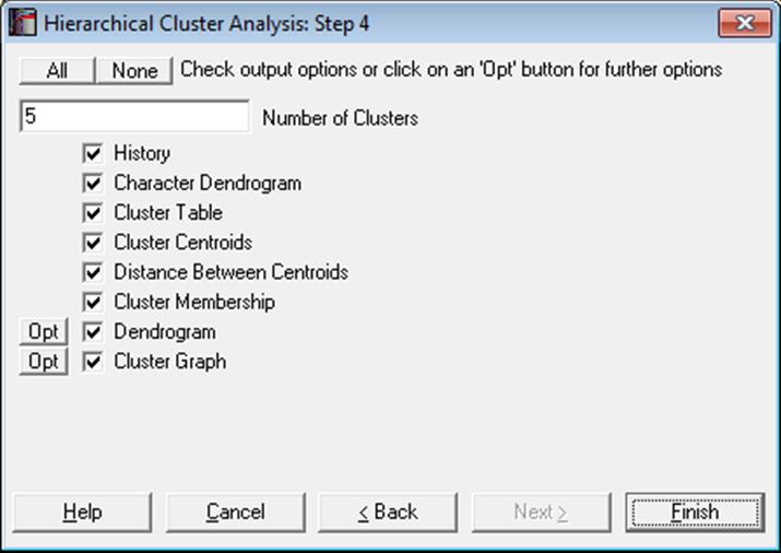
If there are n valid cases in data, the program will start with n clusters and combine them one-by-one until there is only one cluster is left. The History output option will summarise the clustering steps and the two dendrogram diagrams will show this entire process. The remaining output options depend on the Number of Clusters parameter defined by the user.
Number of Clusters: By entering a number between 1 and n, it is possible to display clustering results for any number of clusters. This number can also be changed from within the Cluster Graph, by selecting the Edit → XY Points dialogue.
History: This table shows the two clusters combined at each step, the number of cases in the new cluster and the distance between them. The newly formed cluster is given the label of the cluster in the left hand column.
Character Dendrogram: A dendrogram displays a visual summary of the clustering process, providing you with an understanding of the groups and proximities inherent in data. The order in which clusters are combined does not necessarily coincide with the order they are drawn on a dendrogram. The dendrogram procedure first rearranges the History table to produce an uncluttered tree diagram. The same tree structure can also be output in the form of a graph.
The advantage of this form of output is in its ability to display all Row Labels without any cluttering. However, due its low resolution on the (horizontal) distance axis, some of the clusters which are too close to each other may not be distinguished.
Cluster Table: The number of cases and their percentages are displayed for the number of clusters defined by the user. The within cluster sum of squares, average, minimum and maximum distance of individual cases from their cluster’s centroid are also displayed.
Cluster Centroids: For each cluster, the coordinates of the cluster centroid are displayed.
Distance Between Centroids: Distance between each pair of cluster centroids is displayed in a square-symmetric table.
Cluster Membership: A table containing all cases displays which case belongs to which cluster. As in the Cluster Table option, the number of clusters to be formed can be selected by the user.
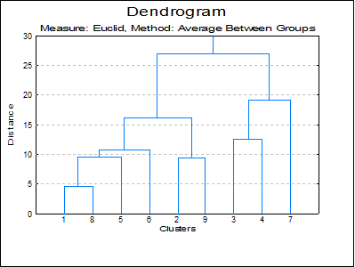
Hi-res Dendrogram: The high-resolution dendrogram is convenient when the number of rows in the data set does not exceed 100. The vertical axis represents the distance and the horizontal axis represents the clusters combined.
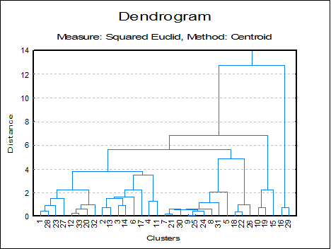
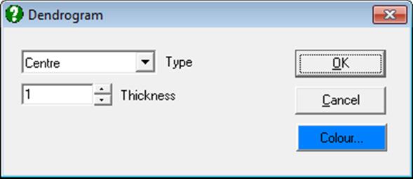
The Edit → XY Points dialogue for the Hi-Res Dendrogram procedure enables you to change the colour and thickness of lines, as well as positions of the stems (the vertical lines representing the newly formed clusters). Stems can be started from the midpoint (the default), the right or the left corner of the line connecting the two old clusters.
By default, the row numbers are displayed as the X-axis labels. It is also possible to display the Row Labels as X-axis labels, from the Edit → Axes dialogue. If the Row Labels are too long, you can display them up and down or rotate the text by 90º or 270º.
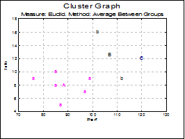
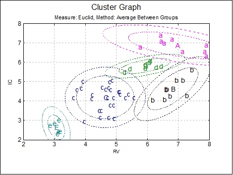
Cluster Graph: Two and three-dimensional scatter diagrams can be displayed showing which data point belongs to which cluster. If you select two variables a 2D graph is displayed and a 3D graph if you select three variables. Different clusters are represented by different letters in different colours.
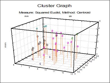
You can change the number of clusters to be displayed from the Edit → XY Points dialogue, without having to go back to the Output Options Dialogue. It is possible to select the font and the size of the letters and display point labels for them. You can also display cluster centroids in capital letters.
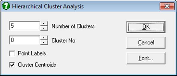
If the Cluster No field is zero, all groups will be displayed simultaneously. If this field is set to any other number less than or equal to the Number of Clusters, then only the cases belonging to that cluster will be displayed.
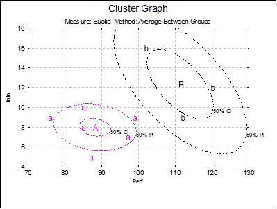
For 2D cluster plots it is also possible to draw ellipse intervals around the cluster centres.
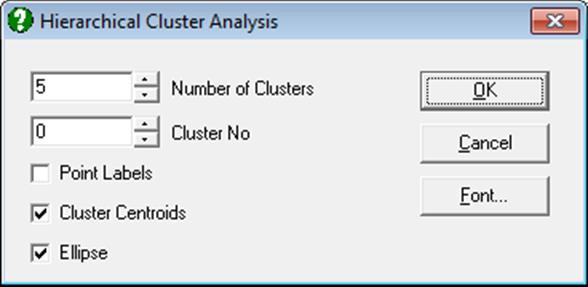
When the Ellipse box is clicked on, the ellipse interval dialog pops up.
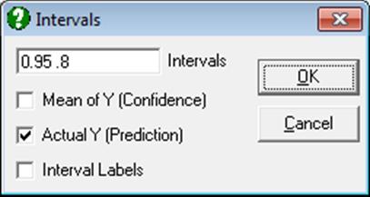
Here you can select multiple confidence levels, which will be drawn for all clusters selected. For further details see Ellipse Confidence and Prediction Intervals in 4.1.1.1.1. Line.
Estimated parameters (correlation coefficient, angle of inclination, two radii and the area enclosed) for all 10 ellipses are saved in the following file:
..\Documents\Unistat10\Work\EllipseInfo.txt
8.1.1.5. Hierarchical Cluster Example
Open MULTIVAR, select Statistics 2 → Cluster Analysis → Hierarchical Cluster Analysis and select Perf, Info, Verbexp and Age (C1 to C4) as [Variable]s. Select distance measure as Euclid and linking method as Average Between Groups. Select number of clusters as 3 and all the output options to obtain the following results:
Hierarchical Cluster Analysis
Variables Selected: Perf, Info, Verbexp, Age
Measure: Euclid, Method: Average Between Groups
History
|
Step |
Combined1 |
Combined2 |
Cases |
Distance |
|
1 |
1 |
8 |
2 |
4.6915 |
|
2 |
2 |
9 |
2 |
9.4345 |
|
3 |
1 |
5 |
3 |
9.5967 |
|
4 |
1 |
6 |
4 |
10.8672 |
|
5 |
3 |
4 |
2 |
12.5714 |
|
6 |
1 |
2 |
6 |
16.1606 |
|
7 |
3 |
7 |
3 |
19.2953 |
|
8 |
1 |
3 |
9 |
26.9553 |
Character Dendrogram
             1+----------+
             8+----------+-----------+
             5+----------------------+--+
             6+-------------------------+-----------+
             2+---------------------+               |
             9+---------------------+---------------+-------------------------+
             3+-----------------------------+                                 |
             4+-----------------------------+---------------+                 |
             7+---------------------------------------------+-----------------+
Cluster Table
|
|
Cases |
Percentage |
Within SSQ |
Average Distance |
Minimum |
Maximum |
|
Cluster 1 |
6 |
66.7% |
479.6467 |
8.2992 |
3.4567 |
12.2459 |
|
Cluster 2 |
2 |
22.2% |
79.0200 |
6.2857 |
6.2857 |
6.2857 |
|
Cluster 3 |
1 |
11.1% |
0.0000 |
0.0000 |
0.0000 |
0.0000 |
Cluster Centroids
|
|
Cluster 1 |
Cluster 2 |
Cluster 3 |
Overall |
|
Perf |
88.1667 |
107.0000 |
120.0000 |
95.8889 |
|
Info |
8.0000 |
12.5000 |
12.0000 |
9.4444 |
|
Verbexp |
32.0000 |
43.5000 |
30.0000 |
34.3333 |
|
Age |
7.1667 |
7.1000 |
8.4000 |
7.2889 |
Distance Between Centroids
|
|
Cluster 1 |
Cluster 2 |
Cluster 3 |
|
Cluster 1 |
0.0000 |
22.5211 |
32.1696 |
|
Cluster 2 |
22.5211 |
0.0000 |
18.7933 |
|
Cluster 3 |
32.1696 |
18.7933 |
0.0000 |
Cluster Membership
|
Observation |
Cluster |
|
1 |
1 |
|
2 |
1 |
|
3 |
2 |
|
4 |
2 |
|
5 |
1 |
|
6 |
1 |
|
7 |
3 |
|
8 |
1 |
|
9 |
1 |
![]()