6.3.1. Chi-Square Tests
One sample and two sample chi-squared tests can be accesses under one menu item and the results will be presented in a single page of output.
If you wish to perform a one sample chi-squared test, you can select only one variable. If you select two or more variables, then two separate one sample tests will be performed on each variable, alongside a two sample test between them. A two sample chi-squared test will be performed only when the two selected [Variable]s have the same length. The Output Options Dialogue will allow you to choose which tests to appear in the output.
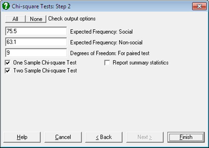
The default expected frequency value suggested by the program is the mean of observed frequencies. These can be changed to any other values. When more than two variables are selected, however, the program does not stop and display the Output Options Dialogue and proceeds with the default expected frequencies.
When the Report summary statistics box is checked, summary information about the selected variables (number of valid cases, missing observations or pairs, mean and standard deviation) is also displayed.
6.3.1.1. One Sample Chi-Square Test
The null hypothesis “observed frequencies are all equal to the given (expected) frequency” is tested. The chi-square statistic is computed as:
![]()
![]()
where foi is the ith observed frequency and fe is the expected frequency.
Example
Example 10.3.1 on p. 529, Larson, H. J. (1982). A die is rolled 200 times and the number of times each number occurs is recorded in a table. The null hypothesis “all six numbers are equally likely” is tested.
Open GOODFIT and select Statistics 1 → Goodness of Fit Tests → Chi-Square Tests. Select Frequency (C1) as [Variable], accept the program’s suggestion of 33.33 as the expected value, check the Report summary statistics box and click [Finish].
Chi-square Tests
|
|
Valid Cases |
Missing |
Mean |
Standard Deviation |
|
Frequency |
6 |
0 |
33.3333 |
1.6330 |
|
|
Expected Frequency |
Chi-Square Statistic |
Degrees of Freedom |
Right-Tail Probability |
|
Frequency |
33.3333 |
2.8600 |
5 |
0.7216 |
This result shows there is no significant difference between the observed frequency and the expected frequency at 5% level. Hence we accept that the likelihood of six numbers are not significantly different.
6.3.1.2. Two Sample Chi-Square Test
This test computes the goodness of fit for two columns containing frequency data. In general, observed frequencies (which are assumed to be in column 1) are compared with expected or theoretical frequencies (which are assumed to be in column 2). Normally, the sums of the two columns are expected to be the same. If this is not the case the program will normalise the values of the second column such that their sum is equal to the first column’s sum. The chi-square statistic is computed as:
![]()
![]()
where foi and fei are the ith observed and expected frequencies respectively.
More than two variables can be selected by clicking on [Variable]. The test will be performed on all possible pairs with equal length. Any pair of cases with at least one missing value is omitted and the degrees of freedom is adjusted.
When a given set of frequencies is compared with a theoretical distribution, allowance should be made in the degrees of freedom for the estimated parameters of the distribution. For instance, if the theoretical distribution (column 2) is normal, the degrees of freedom for the test should be n – 3, to reflect the effect of the estimated distribution parameters, mean and standard deviation. For a Poisson distribution the degrees of freedom is n – 2, as the mean of the distribution should be estimated. To find out about degrees of freedom for other distributions see Appendix.
If only two variables are selected, then the program will prompt for the degrees of freedom, displaying a default value of n – 1. If more than two variables are selected, the program uses this value for all pairs of variables and does not prompt for user input.
The output includes the chi-square statistic, degrees of freedom and the right tail probability.
Example
Example 11.1 on p. 395 from Armitage & Berry (1994). The first column of data contains the observed frequencies of bacterial counts and the second expected frequencies from Poisson distribution.
Open GOODFIT and select Statistics 1 → Goodness of Fit Tests → Chi-Square Tests. Select Observed (C2) as the first variable and Expected (C3) as the second. Enter the degrees of freedom as 6 (instead of the suggested 7 since the Poisson distribution uses 1 parameter), to obtain the following results:
Chi-square Tests
|
|
Valid Cases |
Missing |
Mean |
Standard Deviation |
|
Observed |
8 |
0 |
50.0000 |
39.2538 |
|
Expected |
8 |
0 |
49.9875 |
36.6127 |
|
Observed – Expected |
8 |
0 |
|
|
|
|
Expected Frequency |
Chi-Square Statistic |
Degrees of Freedom |
Right-Tail Probability |
|
Observed |
50.0000 |
215.7200 |
7 |
0.0000 |
|
Expected |
49.9875 |
187.7151 |
7 |
0.0000 |
|
Observed – Expected |
|
6.0150 |
6 |
0.4215 |
This result shows there is no significant difference between the observed and the expected frequencies, though they are both significantly different from zero.