10.2. Slope Ratio Method
This is a general purpose procedure that can be used to analyse balanced or unbalanced assays with blanks (0-dose treatments), plate (row) effects and unlimited numbers of dose levels and test preparations. The algorithm is based on Finney (1978). The Slope Ratio Method specification given in European Pharmacopoeia (1997-2017) is a restricted special case of this procedure.
10.2.1. Slope Ratio Variable Selection
The data format is as in Parallel Line Method (see 10.0.1. Data Preparation and 10.0.2. Doses, Dilutions and Potency). Measurement data is stacked in a single column, a second column contains the dose level for each measurement and another categorical column indicates which preparation a particular measurement belongs to. An optional plate factor can be entered to keep track of plates or replicates.
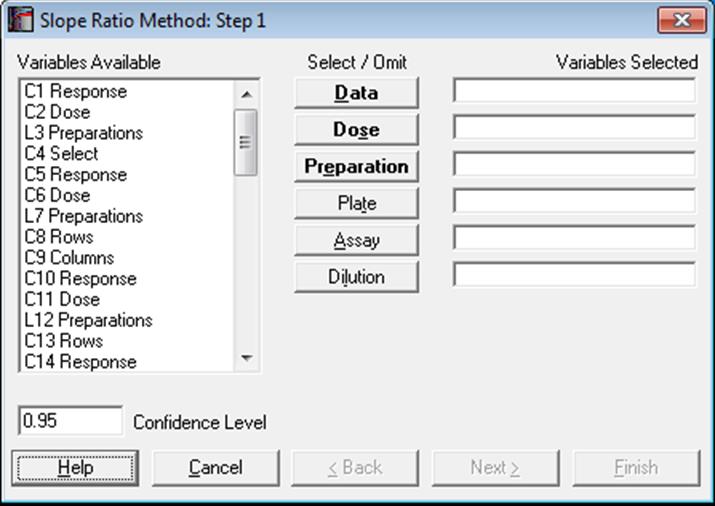
Designs can be unbalanced, i.e. the number of replicates for each dose-preparation combination may be different, dose levels for standard and test preparations may be different, there can be more than one test preparation, but the first five characters of the standard preparation label should be “stand” or “refer” in any language (capitalisation is not significant). Otherwise the first preparation encountered in the [Preparation] column will be considered as the standard (with the exception of blanks). It is compulsory to select at least three columns [Data], [Dose] and [Preparation], which have bold button fonts. The optional [Plate] variable is usually used to isolate a plate effect (or replicates). If all dose/treatment groups (or cells) have an equal number of replicates, or if the design is balanced, then the plate effect is equivalent to Randomised Block Design. For the other two optional variables [Assay] and [Dilution], see sections 10.0.4. Multiple Assays with Combination and 10.0.2. Doses, Dilutions and Potency respectively.
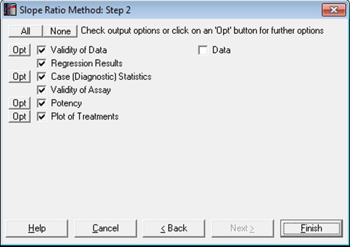
10.2.2. Slope Ratio Output Options
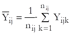
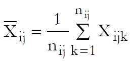
Let Xijk and Yijk be the dose and response values for the ith preparation (i = Blank, Standard, Test 1, …, Test n – 1) and the jth dose level of the kth replicate.
10.2.2.1. Validity of Data
This menu item is identical to the same one available under Parallel Line Method. For details see section 10.1.2.1. Validity of Data.
10.2.2.2. Regression Results
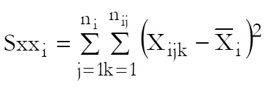
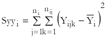
Calculate for i = S, T1, …, Tn – 1:
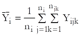
![]()
The estimated parameters of the line of best fit for each preparation (i = S, T1, …, Tn – 1) are:
Slope: ![]()
R-squared: ![]()
Residual sum of squares: ![]()
Standard error of slope: ![]()
This information is displayed in the Separate Regression table and used in drawing the best fit lines in Plot.
The Common Regression is obtained from a multivariate regression run, after transforming the data into the following form first.
|
|
Dependent |
Independent Variables |
||
|
|
Variable |
Standard |
Test 1 |
Test n |
|
Blank |
Y0jk |
0 |
0 |
0 |
|
Replicates |
… |
… |
… |
… |
|
Standard |
YSjk |
XSjk |
0 |
0 |
|
Replicates |
… |
… |
… |
… |
|
Test 1 |
Y1jk |
0 |
X1jk |
0 |
|
Replicates |
… |
… |
… |
… |
|
Test n |
Ynjk |
0 |
0 |
Xnjk |
|
Replicates |
… |
… |
… |
… |
The estimated parameters are displayed in Common Regression table.
10.2.2.3. Case (Diagnostic) Statistics
10.2.2.4. Validity of Assay
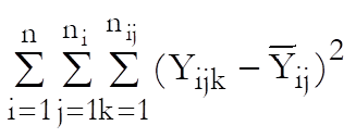
This output option displays an Analysis of Variance (ANOVA) table, which is used in testing the Validity of Assay. The standard significance tests performed are (i) regression, (ii) intercept and (iii) non-linearity. The overall non-linearity test is also broken down to individual tests for each preparation. If blanks (entries with a 0 dose level) exist, there will be an additional term for them. If a [Row Factor] was selected it will appear in the table as a main effect.
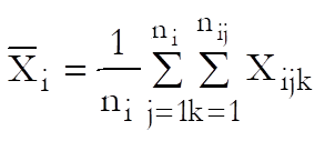
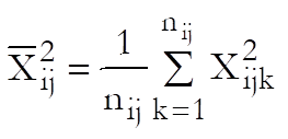
Define a cell as a unique combination of dose levels and preparations. For each cell calculate:
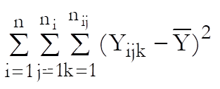
Define the overall mean as:
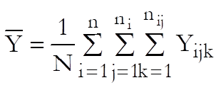
where N is the total number of observations. Also define ![]() and
and ![]() as
the intercept and slope for each preparation from Separate
Regression and
as
the intercept and slope for each preparation from Separate
Regression and ![]() as the slope for
each preparation from Common Regression (see 10.2.2.2. Regression Results).
as the slope for
each preparation from Common Regression (see 10.2.2.2. Regression Results).
The following definitions are used in calculating the blanks effect:
![]()
where Sxxi is as defined in Separate Regression and:
![]()
Also define the number of unique dose-preparation combinations excluding blanks as:
![]()
The ANOVA table is then constructed as follows.
|
Due to |
Degrees of Freedom |
|
Sum of Squares |
|
Plate |
K – 1 |
SSP |
|
|
Between Doses |
D – 1 + B |
SSD |
|
|
Blanks |
B = 0 or 1 |
SSB |
|
|
Regression |
n |
SSR |
|
|
Intercept |
n – 1 |
SSD – SSB – SSR – SSL |
|
|
Non-linearity |
D – 2n |
SSL |
|
|
Non-linearity for Preparationi |
D / n – 2 |
SSLi |
|
|
Residual |
N – D – B – (K – 1) |
SSE – SSP |
– SSP |
|
Total |
N – 1 |
SST |
|
10.2.2.5. Potency
For each test preparation, the potency ratio is calculated as follows:
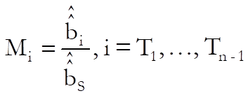
For confidence intervals of M first define Vss, Vii, Vsi, i = T1, …, Tn – 1 as the values corresponding to elements of (X’X)-1 matrix from the Common Regression run. First define:
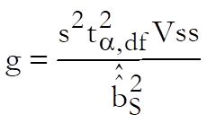
where s2 is the residual mean squares and ![]() is the critical value from the
t-distribution with degrees of freedom of the overall residual term from the
ANOVA table. Note that if divided by s2, Vss, Vii, Vsi give the
variance / covariance matrix of the Common Regression
coefficients.
is the critical value from the
t-distribution with degrees of freedom of the overall residual term from the
ANOVA table. Note that if divided by s2, Vss, Vii, Vsi give the
variance / covariance matrix of the Common Regression
coefficients.
Then the confidence interval for potency ratio of each test preparation is calculated using Fieller’s Theorem (see Finney 1978, p. 156):
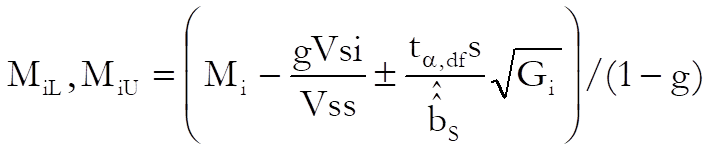
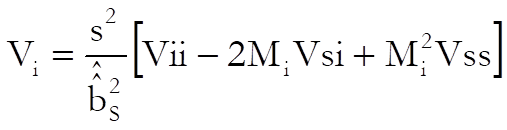
where the variance of Mi is:
![]()
and the approximate variance of Mi is (when g is negligible):
Mi is the relative potency and MiL and MiU are the confidence limits for the relative potency. The estimated potency and its confidence interval are obtained by multiplying these relative values by the assumed potency supplied by the user for each test preparation separately.
Weights are computed after the estimated potency and its confidence interval are found:
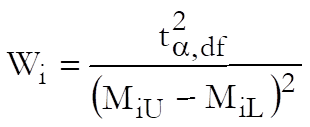
and % Precision is:
![]()
If the data column [Dose] contains the actual dose levels administered in original dose units, we will obtain the estimated potency and its confidence limits in the same units. If, however, the [Dose] column contains unitless relative dose levels, then we may need to perform further calculations to obtain the estimated potency in original units. To do that you can enter assigned potency of the standard, assumed potency of each test preparation and pre-dilutions for all preparations including the standard in a data column and select it as [Dilution] variable. UNISTAT will then calculate the estimated potency as described in section 10.0.2. Doses, Dilutions and Potency. Also see section 10.0.3. Potency Calculation Example.
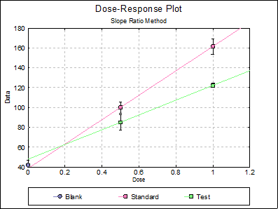
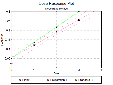
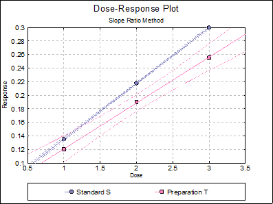
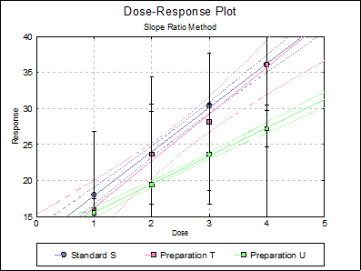
10.2.2.6. Dose-Response Plot
By default, this option generates a plot of treatment means against dose, with standard error bars for each mean. Each preparation will be plotted as one data series, with as many points as the number of doses applied. A line of best fit and its confidence limits will be drawn for each series. This provides a visual means of inspecting the data, enabling the user to notice immediately whether there is something substantially wrong with the data.
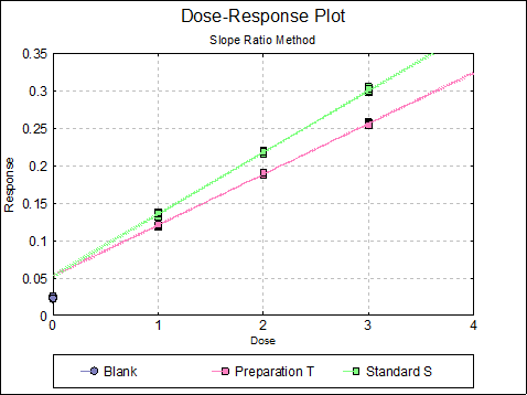
Alternatively, individual response values can be plotted against dose, all with or without trend lines and confidence intervals.
Clicking the [Opt] button situated to the left of Dose-Response Plot output option will place the graph in UNISTAT’s Graphics Editor. Here, all aspects of the graph can be edited and customised.
Selecting Edit → Dose-Response Plot… (or double-clicking on the graph area) will pop a dialogue where what is displayed on the plot can be controlled.
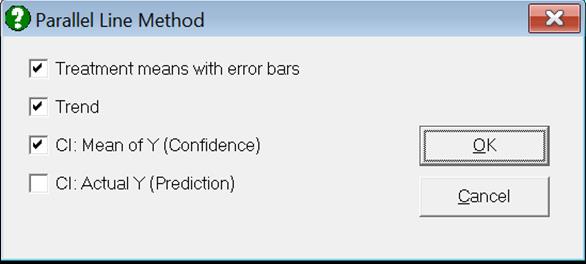
If you uncheck the Treatment means with error bars box, individual response values will be plotted against dose.
10.2.3. Slope Ratio Examples
Example 1
Data is given in Table 5.2.1-I on p. 4369 of European Pharmacopoeia (9th Edition). The data is rearranged as described in section 10.0.1. Data Preparation and saved in columns 27-29 of BIOPHARMA9.
Although the data set contains blanks (0 dose treatments), European Pharmacopoeia (9th Edition ) reports results without blanks. To remove blanks from the analysis, in Excel Add-In Mode, you can simply select the block X10:Z57. In Stand-Alone Mode, you can define C30 as a Select Row column to omit these rows from the analysis, without actually deleting them from the spreadsheet. To do this, click somewhere on column 30, and select Data → Select Row option from UNISTAT’s spreadsheet menus. The colour of C30 will change. This indicates that all rows with a 0 entry in this column will be omitted from subsequent analyses.
Select Bioassay → Slope Ratio Method. In Stand-Alone Mode select columns C27, C28 and L29 respectively as [Data], [Dose] and [Preparation] from the Variable Selection Dialogue. In Excel Add-In Mode, you will need to select the three highlighted columns in the same order. Click [Next] to proceed to Output Options Dialogue. If you do not want to display all normality tests click on the [Opt] button situated to the left of Validity of Data option. Uncheck the tests you do not wish to include in the report. Then click [Back] and [Finish].
In Stand-Alone Mode, do not forget to reset column C30 after you finish this example, otherwise the Select Row function will be effective in subsequent procedures you run. To do this, click somewhere on column C30, and select Data → Select Row option again, or select Formula → Quick Formula from the menu and enter data. The colour of C30 will change back to its original value.
Slope Ratio Method
Rows 1-8 Omitted
Selected by C30 Select
Valid Number of Cases: 48, 8 Omitted
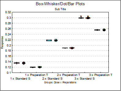
Summary Statistics
Data variable: Response
Subsample selected by: Dose x Preparations
|
|
Valid Cases |
Mean |
Variance |
Standard Error |
|
1 x Standard S |
8 |
0.1351 |
0.0000 |
0.0009 |
|
1 x Preparation T |
8 |
0.1200 |
0.0000 |
0.0004 |
|
2 x Standard S |
8 |
0.2176 |
0.0000 |
0.0007 |
|
2 x Preparation T |
8 |
0.1897 |
0.0000 |
0.0004 |
|
3 x Standard S |
8 |
0.2996 |
0.0000 |
0.0009 |
|
3 x Preparation T |
8 |
0.2554 |
0.0000 |
0.0006 |
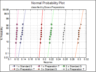
Anderson-Darling Normality Test
Alpha = 0.05
|
Dose x Preparations |
Test Statistic |
Probability |
Pass/Fail |
|
1 x Standard S |
0.4529 |
0.1958 |
Pass |
|
2 x Standard S |
0.3924 |
0.2868 |
Pass |
|
3 x Standard S |
0.6980 |
0.0410 |
**Fail** |
|
1 x Preparation T |
0.5178 |
0.1280 |
Pass |
|
2 x Preparation T |
0.7702 |
0.0258 |
**Fail** |
|
3 x Preparation T |
0.3484 |
0.3758 |
Pass |
Homogeneity of Variance Tests
For 6 groups defined by Dose x Preparations.
Alpha = 0.05
|
|
Test Statistic |
Probability |
Pass/Fail |
|
Levene’s F Test |
2.2830 |
0.0635 |
Pass |
Grubbs’ Outlier Test
Alpha = 0.05
One-tailed tests
|
Dose x Preparations |
Grubbs’ G |
Table G |
Pass/Fail |
|
1 x Standard S G(Min) |
1.6668 |
2.0317 |
Pass |
|
G(Max) |
1.1617 |
2.0317 |
Pass |
|
2 x Standard S G(Min) |
1.2706 |
2.0317 |
Pass |
|
G(Max) |
1.1496 |
2.0317 |
Pass |
|
3 x Standard S G(Min) |
0.9834 |
2.0317 |
Pass |
|
G(Max) |
2.0137 |
2.0317 |
Pass |
|
1 x Preparation T G(Min) |
1.8708 |
2.0317 |
Pass |
|
G(Max) |
0.9354 |
2.0317 |
Pass |
|
2 x Preparation T G(Min) |
1.5022 |
2.0317 |
Pass |
|
G(Max) |
1.0730 |
2.0317 |
Pass |
|
3 x Preparation T G(Min) |
1.3435 |
2.0317 |
Pass |
|
G(Max) |
1.4849 |
2.0317 |
Pass |
G = Maximum deviation from mean / Standard Deviation
Separate Regression
|
|
Intercept |
Slope |
Residual SS |
R-squared |
|
Standard S |
0.0530 |
0.0822 |
0.0001 |
0.9989 |
|
Preparation T |
0.0530 |
0.0677 |
0.0001 |
0.9992 |
Common Regression
|
|
Intercept |
Slope |
Residual SS |
R-squared |
|
Standard S |
0.0530 |
0.0822 |
0.0002 |
0.9990 |
|
Preparation T |
|
0.0677 |
|
|
|
Residual Variance = |
0.0000 |
|
Degrees of Freedom = |
45 |
Validity of Assay
|
Due To |
Sum of Squares |
DoF |
Mean Square |
F-Stat |
Prob |
|
Regression |
0.192 |
2 |
0.096 |
24849.565 |
0.0000 |
|
Intercept |
0.000 |
1 |
0.000 |
0.001 |
0.9780 |
|
Non-linearity |
0.000 |
2 |
0.000 |
2.984 |
0.0614 |
|
Standard S Non-linearity |
0.000 |
1 |
0.000 |
0.086 |
0.7702 |
|
Preparation T Non-linearity |
0.000 |
1 |
0.000 |
5.882 |
0.0197 |
|
Treatments |
0.192 |
5 |
0.038 |
|
|
|
Residual |
0.000 |
42 |
0.000 |
|
|
|
Total |
0.192 |
47 |
0.004 |
|
|
Potency
|
|
Estimated Potency |
Lower 95% |
Upper 95% |
|
Preparation T |
0.8231 |
0.8171 |
0.8292 |
|
|
Relative Potency |
Lower 95% |
Upper 95% |
|
Preparation T |
82.31% |
81.71% |
82.92% |
|
|
Percent CI |
Lower 95% |
Upper 95% |
|
Preparation T |
100.00% |
99.26% |
100.74% |
|
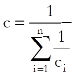
G = |
0.0001 |
|
C = |
1.0001 |
Example 2
Data is given in Table 5.2.2-I on p. 4370 of European Pharmacopoeia (9th Edition).
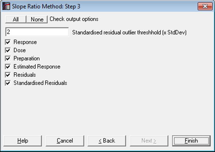
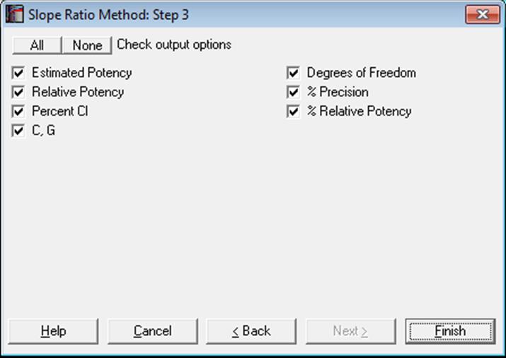
Open BIOPHARMA9 and select Bioassay → Slope Ratio Method. The blank preparation is already omitted from this data set. From the Variable Selection Dialogue select columns C31, C32, L33 and L34 respectively as [Data], [Dose], [Preparation] and [Dilution]. Click [Next] to proceed to Output Options Dialogue. Select the output options below and then click [Finish].
Slope Ratio Method
Valid Number of Cases: 24, 0 Omitted
Separate Regression
|
|
Intercept |
Slope |
Residual SS |
R-squared |
|
Standard S |
11.7500 |
6.1200 |
2.2960 |
0.9939 |
|
Preparation T |
9.7250 |
6.4950 |
13.4085 |
0.9692 |
|
Preparation U |
11.6500 |
3.9200 |
2.1760 |
0.9860 |
Common Regression
|
|
Intercept |
Slope |
Residual SS |
R-squared |
|
Standard S |
11.0417 |
6.3561 |
21.3544 |
0.9807 |
|
Preparation T |
|
6.0561 |
|
|
|
Preparation U |
|
4.1228 |
|
|
|
Residual Variance = |
1.0677 |
|
Degrees of Freedom = |
20 |
Validity of Assay
|
Due To |
Sum of Squares |
DoF |
Mean Square |
F-Stat |
Prob |
|
Regression |
1087.665 |
3 |
362.555 |
339.498 |
0.0000 |
|
Intercept |
3.474 |
2 |
1.737 |
1.626 |
0.2371 |
|
Non-linearity |
5.065 |
6 |
0.844 |
0.791 |
0.5943 |
|
Standard S Non-linearity |
0.446 |
2 |
0.223 |
0.209 |
0.8144 |
|
Preparation T Non-linearity |
4.453 |
2 |
2.227 |
2.085 |
0.1670 |
|
Preparation U Non-linearity |
0.166 |
2 |
0.083 |
0.078 |
0.9257 |
|
Treatments |
1096.205 |
11 |
99.655 |
|
|
|
Residual |
12.815 |
12 |
1.068 |
|
|
|
Total |
1109.020 |
23 |
48.218 |
|
|
Potency
Assigned potency of Standard S: 39 µg HA/ml
Assumed potency of Preparation T: 15 µg HA/dose
Assumed potency of Preparation U: 15 µg HA/dose
|
|
Estimated Potency |
Lower 95% |
Upper 95% |
|
Preparation T |
14.2920 |
13.3681 |
15.2711 |
|
Preparation U |
9.7295 |
8.8542 |
10.6088 |
|
|
Relative Potency |
Lower 95% |
Upper 95% |
|
Preparation T |
95.28% |
89.12% |
101.81% |
|
Preparation U |
64.86% |
59.03% |
70.73% |
|
|
Percent CI |
Lower 95% |
Upper 95% |
|
Preparation T |
100.00% |
93.54% |
106.85% |
|
Preparation U |
100.00% |
91.00% |
109.04% |
|
G = |
0.0056 |
|
C = |
1.0056 |
Example 3
Table 7.10.2. on p. 161 from Finney, D. J. (1978) is an example with blanks, four replicates and two preparations.
Open BIOFINNEY and select Bioassay → Slope Ratio Method. From the Variable Selection Dialogue select columns C12 Data, C13 Dose and S14 Preparations respectively as [Data], [Dose] and [Preparation]. Click [Next] to proceed to Output Options Dialogue. Click [All] to select all output options and then click [Finish]. The potency ratio and its confidence limits are calculated with the default assumed potency of 1. The following output is obtained.
Slope Ratio Method
Valid Number of Cases: 20, 0 Omitted
Separate Regression
|
|
Intercept |
Slope |
Residual SS |
R-squared |
|
Standard |
38.5000 |
123.0000 |
111.0000 |
0.9855 |
|
Test |
47.7500 |
74.5000 |
72.7500 |
0.9745 |
Common Regression
|
|
Intercept |
Slope |
Residual SS |
R-squared |
|
Standard |
42.1429 |
118.6286 |
252.8857 |
0.9920 |
|
Test |
|
81.2286 |
|
|
|
Residual Variance = |
14.8756 |
|
Degrees of Freedom = |
17 |
Validity of Assay
|
Due To |
Sum of Squares |
DoF |
Mean Square |
F-Stat |
Prob |
|
Regression |
31456.914 |
2 |
15728.457 |
1089.731 |
0.0000 |
|
Blanks |
2.161 |
1 |
2.161 |
0.150 |
0.7043 |
|
Intercept |
34.225 |
1 |
34.225 |
2.371 |
0.1444 |
|
Non-linearity |
0.000 |
0 |
|
|
|
|
Treatments |
31493.300 |
4 |
7873.325 |
|
|
|
Residual |
216.500 |
15 |
14.433 |
|
|
|
Total |
31709.800 |
19 |
1668.937 |
|
|
Potency
|
|
Estimated Potency |
Lower 95% |
Upper 95% |
|
Test |
0.6847 |
0.6464 |
0.7236 |
|
G = |
0.0021 |
|
C = |
1.0021 |