Time Series Analysis-Browns Exponential - Unistat Statistics Software

UNISTAT - the ultimate Excel statistics add-in

This simply calculates the exponential weighted average in time. For a data series xt forecasts are given by:

where:

· is the level at time t.

· is the level smoothing constant.

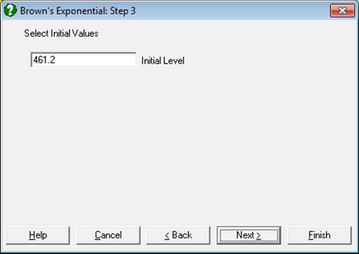
Time Series Analysis-Browns Exponential

The initial value m0 is calculated as the average level in the first quarter of the series.

Time Series Analysis-Browns Exponential

Example

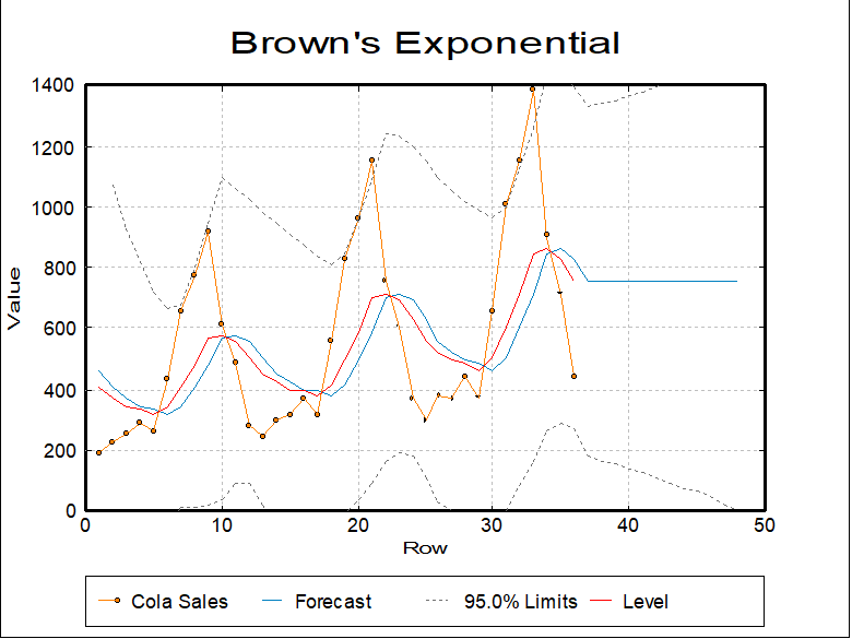
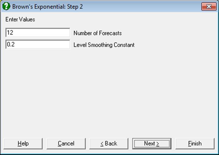
Open TIMESER and select Statistics 2 → Forecasting → Brown’s Exponential and select Wald Statistic

(C2) as [Variable]. On the following dialogues accept the program’s sugestions:

Brown's Exponential

Level Smoothing Constant =	0.2000
Sum of Squares =	3029058.7929

Summary Table

Time Series Analysis-Browns Exponential